
ML Interview Q Series: Can you describe the three main classifications of anomaly detection methods?


📚 Browse the full ML Interview series here.
Comprehensive Explanation
Anomaly detection is the practice of identifying unusual patterns or outliers in data that do not align with normal distributions or expected behaviors. The three major approaches are typically supervised, unsupervised, and semi-supervised.
Supervised anomaly detection relies on labeled datasets where examples of both normal instances and anomalies are available. This approach involves training a classifier to recognize anomalies based on known examples. In practice, acquiring labeled anomaly samples can be difficult because anomalies are often rare or previously unknown.
Unsupervised anomaly detection does not require labels. The assumption here is that most data points fall into a “normal” region, so any data instance that appears to deviate significantly from this normal structure is considered anomalous. Methods under this approach often leverage clustering or density-based techniques. When no labeled data is available at all, unsupervised methods are often the only option.
Semi-supervised anomaly detection lies in between. It typically uses labeled examples of normal behavior and no labeled anomalies. The model tries to capture the properties of normal data and then flags anything that deviates notably. This approach can be more effective than purely unsupervised methods because it leverages knowledge about what normal data looks like, yet it does not require labeled outliers.
One popular technique for anomaly detection is the use of reconstruction-based methods, such as autoencoders. An autoencoder is trained to reconstruct normal data. When an anomaly is fed into this model, it yields a reconstruction significantly different from the input if the model has only ever seen normal examples.
Below is a common objective function used in autoencoder-based anomaly detection, where E(x) is the reconstruction error:
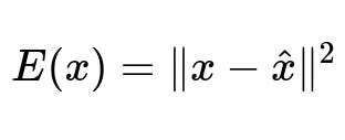
In this expression, x represents the original input data point, and x_hat is the reconstructed data from the autoencoder. If E(x) exceeds a threshold, x is flagged as an anomaly. This method works especially well if you can acquire a clean dataset of normal samples (semi-supervised setting) for training the autoencoder.
Possible Implementation Details
When implementing supervised anomaly detection, you typically use a labeled dataset, training a classifier (e.g., SVM, Random Forest, or deep neural networks) on both normal and anomalous classes. If anomalies are extremely rare, techniques such as synthetic oversampling or class-weighted losses can be applied to deal with class imbalance.
For unsupervised approaches, you might apply clustering-based (e.g., DBSCAN) or density-based (e.g., Kernel Density Estimation) algorithms. Points that do not belong to any cluster or are in low-density regions might be viewed as anomalies. Another unsupervised approach is an Isolation Forest, which isolates anomalies by recursively partitioning the data space.
In a semi-supervised pipeline, you would often train a model on purely normal data. After obtaining a model of “normality” (e.g., an autoencoder or a One-Class SVM), you score new points by their deviation from normal patterns. A high deviation suggests an anomaly.
Edge Cases and Practical Considerations
In supervised settings, anomalies might evolve over time. A model trained on older data could fail to detect novel anomalies. Periodic retraining or online learning can mitigate this.
Unsupervised techniques can be sensitive to hyperparameter choices, such as the number of clusters or density thresholds. Improper tuning can either over-flag normal instances or miss true anomalies.
Semi-supervised methods rely on the assumption that you have only normal data during training. If anomalies unintentionally creep into the training set, the model could learn a skewed representation of what is “normal.”
Finally, real-world data often contain noise, missing values, and complex distributions. Combining domain knowledge with robust data preprocessing is crucial for reliable anomaly detection.
How to Validate Performance
Validating anomaly detection can be challenging when anomalies are hard to label. In supervised or partially supervised contexts, standard metrics like precision, recall, and the F1 score can be used. In an unsupervised scenario, domain experts may have to verify flagged anomalies, or you can use synthetic anomaly injection on real data for evaluation.
Follow-up Questions
What is the difference between outlier detection and novelty detection?
Outlier detection typically deals with data points that fall outside the normal distribution in a static dataset. Novelty detection often focuses on identifying anomalies in a streaming context, meaning the model is constantly updated as new data arrives. Novelty detection aims to detect unforeseen patterns not present in the training distribution. In outlier detection, you usually assume all anomalies are already in the dataset.
How does an Isolation Forest method identify anomalies?
Isolation Forest randomly partitions feature values, repeatedly splitting data into subsets. Because anomalies are typically scarce and different from normal points, they get isolated faster, requiring fewer splits to separate them from the rest. The method computes an “isolation” score for each point: a higher score indicates that point is easier to isolate and hence more likely an anomaly.
Could we use deep learning models other than autoencoders for anomaly detection?
Yes. Other models such as Generative Adversarial Networks (GANs) or transformer-based architectures can be adapted for anomaly detection. For instance, GAN-based methods might generate data that resemble the normal class, and anomalies yield high discriminator scores. In sequence data settings, transformer-based models can learn normal sequences and assign elevated reconstruction errors or likelihood deviations to anomalous sequences.
When might a purely supervised approach be infeasible?
A purely supervised approach relies on having examples of anomalies labeled in the training set. In many practical situations, anomalies are extremely rare or diverse, and you might not have prior knowledge of their variations. This makes it hard to gather labeled examples, so a purely supervised approach may fail to detect unseen anomaly types. Semi-supervised or unsupervised methods are more suitable in these cases.
How do you handle unbalanced data in supervised anomaly detection?
You can modify the training process with techniques such as class weighting, adjusting the loss function to penalize misclassifications of anomalies more heavily. Alternatively, oversampling methods like SMOTE can synthetically create more examples of the minority (anomalous) class. However, synthetic data might not always be realistic for anomalies, so domain knowledge should guide these decisions.
How do you pick a threshold for reconstruction error?
A common practice is to calculate reconstruction errors on a validation set (assumed to contain normal samples) and decide a threshold based on statistical percentiles (for example, the 95th or 99th percentile of errors). Another approach is to use domain knowledge or label information (if available) to optimize the threshold for specific metrics like the F1 score or a target false positive rate.
Below are additional follow-up questions
How does concept drift affect anomaly detection, and what strategies can address it?
Concept drift occurs when the statistical properties of data change over time in ways not captured by the model. In anomaly detection, a model that was once accurate might start misclassifying normal data as anomalies if the “normal” patterns change. Alternatively, new forms of anomalies might arise that the model fails to detect. This drift can be gradual (small changes accumulate over time), sudden (distribution changes abruptly), or recurring (patterns repeat at different intervals).
To handle concept drift in anomaly detection, one approach is to implement online or incremental learning algorithms that continually update model parameters as new data arrives. Another strategy is to use a sliding window or a forgetting mechanism that discards outdated data points. Additionally, regularly retraining or fine-tuning on more recent data can help the model adapt to new patterns. However, a subtle pitfall is overfitting to recent data and losing the broader contextual understanding of past anomalies, which might still be relevant.
How can we evaluate anomaly detection models when the ground truth is uncertain or nonexistent?
In many real-world scenarios, obtaining a ground-truth label for anomalies is difficult because anomalies are rare, expensive to label, or may not have occurred in historical data. Without reliable ground truth, common metrics like accuracy, precision, and recall become less straightforward to apply.
One practical strategy is to simulate anomalies in a controlled setting to produce synthetic or “proxy” ground truth. Though these synthetic anomalies may not perfectly reflect real anomalies, they can still help in model assessment. Another approach is to rely on domain experts who can qualitatively verify the anomalies flagged by the model. Crowdsourcing might be an option in cases where domain expertise can be scaled. Yet a major pitfall is relying solely on synthetic anomalies that might bias the model toward a specific type of outlier, ignoring other forms that occur in reality.
How do high-dimensional datasets impact anomaly detection, and what techniques help mitigate the curse of dimensionality?
As the dimensionality of data increases, distance metrics become less meaningful, and density estimation becomes harder. This phenomenon, known as the curse of dimensionality, can cause traditional anomaly detection algorithms (e.g., distance-based or density-based methods) to perform poorly. Anomalies may blend into the data, making it challenging to differentiate them from normal points.
Dimensionality reduction techniques like PCA, t-SNE, or autoencoders can help capture the most relevant structure in a lower-dimensional space, making anomalies easier to spot. Feature selection methods driven by domain knowledge can also reduce dimensionality by retaining only the features most relevant to anomaly detection. A pitfall is over-reduction: if the dimensionality is reduced too aggressively, subtle but critical signals that indicate anomalies may be lost.
How can time-series and temporal dependencies be leveraged for anomaly detection?
When data points are sequential (e.g., sensor readings over time), simply treating each point independently can miss vital information about trends and patterns. Models such as recurrent neural networks (RNNs), LSTMs, or Temporal Convolutional Networks (TCNs) can capture temporal dependencies, learning how a sequence typically evolves and flagging departures from these expected trajectories.
A challenge arises when the seasonal patterns or trends drift over time, making older segments less representative of the current behavior. Properly handling these time-varying factors may require periodic retraining or adopting adaptive models that capture changing seasonal effects (e.g., a daily or yearly cycle). Another edge case is multi-step forecasting, in which you predict future values and treat large forecast errors as potential anomalies; however, inaccurate forecasts could increase false positives if the forecasting model is not robust.
What roles do domain knowledge and business context play in anomaly detection?
Purely data-driven models can flag anomalies based on statistical rarity, but in practice, not every rare event is an anomaly of concern. Domain knowledge or business context can help differentiate innocuous “strange” events from genuinely problematic ones. For instance, in network intrusion detection, an unusual traffic pattern might be a harmless software update or an actual attack. Subject-matter experts can guide the setup of rules or define special features that better characterize normal and abnormal behaviors.
A hidden risk is over-reliance on domain knowledge that might become outdated. Experts might impose rules that reflect past conditions but ignore evolving behaviors or new threats. Thus, combining expert input with regular data-driven updates keeps the anomaly detection system relevant over time.
How do parametric vs. non-parametric methods differ in anomaly detection, and when might you choose each?
Parametric methods assume the data follows a known distribution (e.g., Gaussian), requiring estimation of a fixed set of parameters. These approaches are often computationally efficient and simpler to interpret. However, they may fail when the true distribution is multimodal or significantly non-Gaussian.
Non-parametric methods make fewer assumptions about the underlying distribution, potentially adapting better to complex data. Examples include kernel density estimation and distance-based approaches. The trade-off is that non-parametric methods can be more computationally intensive, especially as the dataset grows. In practice, if domain knowledge or prior analysis suggests the data roughly follows a known distribution, a parametric model might be both simpler and accurate. Otherwise, a non-parametric or hybrid approach is more robust but requires careful tuning to avoid overfitting in high dimensions.
How can anomaly detection systems function in real-time for streaming data?
Real-time or streaming anomaly detection involves processing data on the fly, flagging anomalies nearly as soon as they appear. One solution is to use incremental algorithms that update their internal representations with every new observation, such as online clustering or online autoencoder variants. Sliding windows or fixed-size buffers help manage memory and remove obsolete data.
The main challenge is ensuring both computational efficiency and consistent performance. If the model updates too frequently, it may overfit the current window and miss broader context. If it updates too slowly, it might fail to detect rapidly changing anomalies. Additionally, sudden spikes in data volume (e.g., in networking logs or sensor streams) can cause delays or lost data. In such scenarios, scaling the system horizontally (e.g., Apache Kafka with Spark Streaming) can handle large flows while maintaining near real-time performance.
How do we provide interpretability and transparency in anomaly detection?
Many anomaly detection models (e.g., deep autoencoders) operate as “black boxes,” producing an anomaly score without clear explanations. In high-stakes domains (finance, healthcare, security), users often need to understand why a particular data point is flagged. One approach is to generate feature-level importance scores, indicating which features most contributed to the anomaly score. Another method is to approximate the model locally using simpler, interpretable models.
A potential pitfall is over-simplifying the explanation, which might mislead stakeholders. For instance, a local approximation might not hold in other regions of the data space. Balancing interpretability with accuracy is key, and domain experts should validate whether these explanations match real-world reasoning about anomalies.
How do we maintain robustness when data is noisy or training labels for anomalies are imperfect?
Real-world data often contains mislabeled points, missing values, or measurement errors. When labels are incorrect—either by mistaking normal instances for anomalies or vice versa—the model can learn an inaccurate decision boundary. Noise in features may further muddle patterns that distinguish normal from abnormal.
To combat label noise, you can use robust loss functions that reduce the impact of outliers in training, or you can apply semi-supervised learning if you are more confident in the normal samples. Imputation techniques or domain-driven cleaning rules can help handle missing or corrupted data. However, a risk is “cleaning away” actual anomalies. An overzealous data-preprocessing pipeline might remove precisely the data points that indicate rare, but critical, anomalies. Thus, data cleaning and robust modeling must be balanced with caution about the possibility of discarding or masking anomalies.
Is it beneficial to combine multiple anomaly detection methods into an ensemble?
In many cases, an ensemble can outperform a single method by leveraging diverse perspectives on the data. For example, an ensemble might combine distance-based and reconstruction-based methods, flagging data points that multiple algorithms independently consider anomalous. This approach can produce more stable and accurate decisions, particularly when dealing with varying types of anomalies.
A common pitfall is poor calibration between different model outputs. If the methods are not normalized or weighted correctly, one method’s high anomaly score could overshadow others. Ensemble approaches can also be computationally expensive. Additionally, interpretability might be reduced if each ensemble component has different criteria for flagging anomalies. To tackle these challenges, one might implement a meta-learner that takes each model’s anomaly score as input and then delivers a final decision.