ML Interview Q Series: Can you use Batch Normalisation in Sparse Auto-encoders?

📚 Browse the full ML Interview series here.

Comprehensive Explanation

Sparse Auto-encoders encourage most hidden units to remain inactive (close to zero) for each input, while only a small fraction of units become active. Typically, the sparseness constraint is introduced by adding a regularization term to the loss function that penalizes deviations of hidden layer activations from a desired sparsity level. In practice, this is often done by measuring the average activation of each hidden neuron over the training set and penalizing large deviations from a target average activation (for instance, 0.05).

A standard form of this penalty uses the Kullback–Leibler (KL) divergence between the desired activation rho and the average activation hat_rho_j for each hidden neuron j:

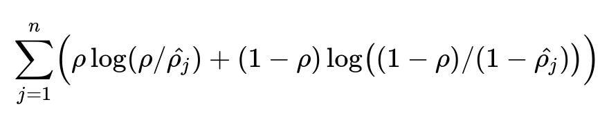
n is the number of neurons in the hidden layer, rho is the desired average activation (a small value such as 0.05), and hat_rho_j is the observed average activation of neuron j. This regularization ensures that neurons remain mostly inactive, thereby enforcing sparsity.

Batch Normalization (BN) is a technique originally introduced to stabilize and accelerate training in deep neural networks by normalizing the inputs to each layer. It computes the mean and variance of the activations across the batch dimension and then applies a learnable shift and scale.

In principle, there is no strict incompatibility between Batch Normalization and the sparsity constraint. You can use both techniques together. However, there are several nuances worth considering.

When BN is applied just after a linear or convolutional transform, it rescales and shifts the activations based on the statistics of the batch. This can sometimes reduce the “natural” skewness of activations that certain regularizers rely on, including sparsity regularizers. If the network heavily relies on sparse representations, BN may at times counteract that by normalizing and shifting each neuron’s activation distribution.

Nevertheless, with careful tuning, including choosing an appropriate momentum, learning rate, and ensuring that the Batch Normalization parameters (gamma and beta) don’t undo the intended sparse activation, it is feasible to incorporate BN into a sparse auto-encoder architecture. In practice, you might observe that training requires more careful hyperparameter selection. Some practitioners choose alternative normalization approaches such as Layer Normalization or Group Normalization when dealing with architectures that rely on strict activation patterns.

Below is a conceptual snippet demonstrating how one might insert Batch Normalization into a sparse auto-encoder in PyTorch.

import torch
import torch.nn as nn
import torch.nn.functional as F

class SparseAutoencoder(nn.Module):
    def __init__(self, input_dim, hidden_dim, sparsity_target=0.05, beta=1.0):
        super(SparseAutoencoder, self).__init__()

        self.encoder = nn.Sequential(
            nn.Linear(input_dim, hidden_dim),
            nn.BatchNorm1d(hidden_dim),  # Insert Batch Norm here
            nn.ReLU()
        )

        self.decoder = nn.Sequential(
            nn.Linear(hidden_dim, input_dim),
            nn.Sigmoid()
        )

        self.sparsity_target = sparsity_target
        self.beta = beta

    def forward(self, x):
        encoded = self.encoder(x)
        decoded = self.decoder(encoded)
        return decoded, encoded

    # Hypothetical loss calculation
    def loss_function(self, x, decoded, encoded):
        # Reconstruction loss
        recon_loss = F.mse_loss(decoded, x, reduction='mean')

        # Calculate average activation for the hidden layer
        p_hat = torch.mean(encoded, dim=0)

        # Sparsity penalty using KL Divergence
        # This is an inline textual representation for demonstration
        # KL(p||p_hat) = p*log(p/p_hat) + (1-p)*log((1-p)/(1-p_hat))
        kl_div = self.sparsity_target * torch.log((self.sparsity_target + 1e-10)/(p_hat + 1e-10)) \
                 + (1 - self.sparsity_target) * torch.log(((1 - self.sparsity_target) + 1e-10)/((1 - p_hat) + 1e-10))
        sparsity_loss = torch.sum(kl_div)

        return recon_loss + self.beta * sparsity_loss

This shows how BN could be placed between the linear transform and the nonlinearity in the encoder. The loss_function calculates both a reconstruction loss and a sparsity penalty. In many scenarios, this combination can work well, but you must tune hyperparameters carefully to ensure that BN does not nullify the intended sparse distribution of activations.

Do we lose the benefits of Batch Normalization if we want to enforce neurons to remain "mostly off"?

Batch Normalization can sometimes make the activations more uniform, which might clash with the idea of having neurons off most of the time. However, the learnable parameters within BN give the network the flexibility to still drive activations towards zero if the training process deems it beneficial. If the final shift and scale learned by BN support that neurons remain close to zero, you will still see sparse-like behavior. So the benefits of BN in stabilizing gradients and improving convergence can still be retained, though care is needed with tuning.

Are there specific best practices when combining BN with sparsity constraints?

One practical approach is to experiment with the location of BN. Some people place BN on only the decoder side or skip BN layers in certain parts of the encoder. Another strategy is to reduce the momentum so that running statistics reflect the desired sparse distribution more accurately. Or you can consider alternative normalization methods that might align better with very low activation regimes, such as Layer Normalization, which normalizes across features rather than across the batch dimension.

Could Batch Normalization mask the effect of the KL Divergence penalty?

If the BN layer shifts and scales activations aggressively, the measured average activation might deviate from what the KL divergence penalty alone would induce. The remedy is to ensure that the scale and shift parameters in BN are not overpoweringly large. Tuning the initial scale parameter (commonly referred to as gamma) can help. Sometimes people initialize gamma to small values so that the network does not overshadow the natural distribution of activations. Monitoring the running statistics of the BN layer and the actual average activations of the hidden neurons can indicate whether BN is hampering sparsity.

Could Layer Normalization or other normalization approaches be more suitable?

Layer Normalization normalizes activations across the feature dimension instead of across the batch. This often makes the training more stable for tasks where batch statistics might interfere strongly with the specialized activation patterns of certain architectures (like sparse auto-encoders dealing with small target activations). In practice, if Batch Normalization doesn’t provide the expected improvements or requires too much delicate tuning, trying Layer Normalization or Group Normalization could be a good alternative.

What happens if the batch size is very small in a sparse setup?

Very small batch sizes can lead to noisy estimates of mean and variance in BN. When the network is also trying to maintain a very low average activation, the noise in the BN statistics may repeatedly shift neurons away from zero, making it harder to enforce stable sparsity. Smaller batch sizes can force BN to rely on running averages, and you must ensure they converge properly. If a stable sparse representation is not observed, either increase batch size or consider switching to a normalization method that does not rely on batch statistics.

How would you debug a sparse auto-encoder with BN that is not producing sparse activations?

You can track the following in a debugging session:

• Monitor the distribution of hidden activations over training epochs. If the average activation is not close to your target, verify that your KL divergence penalty (or other sparsity regularization) is not too small or overshadowed by the reconstruction loss.

• Track Batch Normalization parameters (running_mean, running_var, and weight/bias if using PyTorch). Check if they are adapting in a way that pushes activations away from zero. Adjusting hyperparameters such as the momentum, initial gamma, or learning rate might help.

• Consider turning off BN momentarily to see if the model can achieve the sparsity you want, then reintroduce it to see the effect.

If adjusting these aspects doesn’t restore sparse behavior, switching to another normalization approach might be more straightforward.

Below are additional follow-up questions

How should the Batch Normalization layers be initialized in a sparse auto-encoder?

A common practice for Batch Normalization (BN) is to initialize the scale parameter (gamma in many frameworks) to 1.0 and the shift parameter (beta) to 0.0. However, in a sparse auto-encoder, where neurons are encouraged to be close to zero most of the time, this default initialization may not always be optimal:

1. Why initialization matters

   • In BN, the parameters gamma and beta control how the normalized activations are scaled and shifted. If gamma is too large, the network might amplify activations that would otherwise be near zero. If beta is too large, it might shift activations away from zero, reducing sparsity.

   • Sparse auto-encoders use a KL-divergence or another penalizing metric to push hidden units toward low activation. If the BN layer has large initial biases or large initial scaling, it may counteract that push.

2. Potential strategies

   • Smaller gamma initialization: Initializing gamma to a value slightly less than 1 (e.g., 0.1–0.5) helps keep activations compressed. This can make it easier for the sparse penalty to keep neurons at a low value.

   • Zero or near-zero beta: Ensuring beta starts near zero prevents shifting the mean activation away from zero initially.

   • Monitor BN stats: After initialization, keep an eye on the running mean and running variance. If they drift significantly, the BN layer might be overriding the sparsity objective, and you may want to adjust the learning rate or re-initialize.

3. Pitfalls

   • Extreme initial values: If gamma is initialized too low (e.g., 0.0001), gradients might vanish because the entire layer’s output becomes very small, making learning difficult.

   • Overly tight focus on zero: If beta is forced to remain at zero and gamma is very small, the model might have trouble learning representations that deviate from zero at all. The auto-encoder might end up in a degenerate solution with trivial outputs.

By experimenting with different initial values for BN parameters, you can balance between giving the network flexibility to learn and preserving the push toward sparse activations.

---

Would it help to freeze the Batch Normalization parameters at some point in training for stable sparse activations?

Freezing BN parameters means stopping the update of both the running mean/variance and the learnable gamma/beta. This can be done partway through training once you believe the BN layers have converged to stable statistics:

1. Why you might freeze BN

   • Stability: If the sparse auto-encoder has already found a regime where the activations hover near the target sparsity, further updates to BN’s running statistics might disturb that equilibrium.

   • Less interference: Freezing BN can help ensure that the fine-tuning of the sparse penalty (KL-divergence) isn’t constantly fighting BN’s evolving normalization.

2. How to do it

   • Monitor training: Watch if the network’s running mean/variance in BN layers stabilizes. If the values oscillate only slightly around some range, it can indicate the BN statistics have largely converged.

   • Manual freeze: In frameworks like PyTorch, you can set requires_grad=False for the BN parameters (weight, bias) and prevent updates to the running statistics by switching the layer into eval() mode (though this also has implications for dropout and other layers in eval() mode).

3. Pitfalls

   • Early freeze: If you freeze BN too soon, you might lock in suboptimal statistics, making it harder for the network to further adjust for better reconstruction or stronger sparsity.

   • Late freeze: If you freeze BN parameters too late, you might not gain any advantage because the network has already settled on the final distribution of activations.

In many cases, letting BN learn throughout training is sufficient, but for certain tricky sparse auto-encoder setups, freezing BN can be an extra tool to maintain stable sparse representations once a good regime is found.

---

Does the placement of Batch Normalization (before or after the activation function) affect sparsity?

In many standard architectures, BN is placed before the nonlinearity (e.g., ReLU). However, some practitioners experiment with placing BN after the nonlinearity. Sparse auto-encoders may see different behaviors depending on this choice:

1. BN before activation

   • Normalized linear outputs: The linear layer outputs are normalized, then passed through the ReLU or another sparse-friendly activation.

   • Effect on sparsity: The ReLU (or any activation) sees mean-zero, unit-variance inputs, which might result in a certain proportion of negative inputs being clipped to zero. This can interact naturally with sparsity, but also might reduce the natural skewness that fosters some units being very close to zero.

2. BN after activation

   • Normalized nonlinear outputs: The activation function’s output is normalized. Because ReLU outputs are zero or positive, the mean might shift differently.

   • Potential conflict: If the BN after ReLU shifts the distribution upward, it might reduce the proportion of zeroes, interfering with the targeted sparsity. On the other hand, if BN learns to shift the distribution close to zero, it might encourage even more zero activations.

3. Pitfalls

   • Vanishing activations: Placing BN after a ReLU might lead to a large fraction of zero values, and then BN sees mostly zero data in certain minibatches, causing unstable variance estimates.

   • Overcorrection: BN might “over-correct” for the spike at zero, artificially boosting a subset of activations above zero.

In practice, the most common arrangement is BN before activation. However, for achieving strong sparsity, it can be valuable to experiment with both placements to see which yields the best synergy with the KL divergence penalty.

---

How do gradient-based optimizers behave with BN in a sparse auto-encoder?

Training a sparse auto-encoder with BN adds extra complexity to the gradient flow because both the linear parameters and the BN parameters (plus the running statistics) are being updated:

1. Key interactions

   • Optimizer momentum: If your optimizer has momentum (e.g., in SGD with momentum), the updates to BN parameters can lag behind the rapidly changing sparse activations. This sometimes causes the effective normalization to mismatch the actual distribution of the activations, especially early in training.

   • Learning rate scheduling: BN layers are sensitive to changes in the scale of gradients. If your learning rate is too high, BN parameters might overshoot their ideal values, destabilizing the training. Conversely, a too-low learning rate may cause extremely slow updates, letting the network remain in a suboptimal zone for longer.

2. Pitfalls

   • Overly high learning rate: This might cause repeated “tug-of-war” between the BN updates and the sparse penalty. The network might oscillate, with BN pulling activations up/down while the penalty tries to push them to zero.

   • Inconsistent batch statistics: If you use something like Adam or RMSProp with small batch sizes, the per-parameter adaptive learning rates can combine with BN’s running means/variances in unpredictable ways. You might see large fluctuations in hidden unit activations, undermining stable sparsity.

3. Practical tips

   • Start with smaller LR: Often, a smaller or well-tuned initial learning rate helps keep BN stable in the presence of a strong sparse regularizer.

   • Gradual warm-up: A short warm-up phase for the learning rate can let BN statistics adapt to the initial data distribution before the strong push for sparsity starts dominating.

Keeping a close eye on the synergy between your chosen optimizer and BN can help the network converge to a balance between reconstruction quality and the desired level of sparsity.

---

How do additional regularization methods (like dropout or weight decay) interact with BN in a sparse auto-encoder?

Many practitioners add dropout or weight decay in auto-encoders to encourage generalization. When BN and a sparsity constraint are also in the mix, the interactions can become complex:

1. Dropout

   • Randomly zeroing activations: If dropout is applied to the hidden layer along with BN, the batch statistics can become noisier since each training step sees a subset of active neurons.

   • Combined effect on sparsity: Dropout already pushes the network to not rely on specific neurons being always active. Coupled with the KL divergence penalty, you might see more extreme sparsity than intended, or the network might struggle to learn meaningful features.

   • Order of operations: Typically, BN is placed before dropout. If you reverse the order, BN will see a partially zeroed set of activations, which can compromise the stability of its running statistics.

2. Weight decay (L2 regularization)

   • Penalizing large weights: This can help reduce the magnitude of the weights in the linear layers, which in turn may indirectly reduce overall activation magnitudes.

   • Interaction with BN: BN layers already help keep outputs within a certain range. If weight decay is too strong, it may push weights close to zero, and combined with BN normalization, the learned representations might become overly restricted.

   • Balancing terms: The relative strength of weight decay, sparse penalty, and BN’s scale/shift parameters must be carefully tuned.

3. Pitfalls

   • Overregularization: Applying dropout, L2 regularization, and a KL divergence for sparsity all at once can cause severe underfitting if any combination is too aggressive.

   • Stochastic interactions: Dropout’s randomness can cause large variations in BN’s computed mean and variance, especially for small batch sizes or extremely sparse layers.

In practice, experiment carefully with each regularization method’s strength and monitor validation reconstruction loss and hidden activation histograms to verify the synergy among all components.

---

Could partial use of BN (e.g., only in the decoder) benefit a sparse auto-encoder?

“Partial BN” refers to applying BN only to specific parts of the network. For instance, you might skip BN in the encoder to preserve raw, potentially skewed activations that facilitate sparsity, but still use BN in the decoder for stable reconstruction:

1. Why partial BN might help

   • Preserve sparsity patterns: The encoder’s first layers are often where the KL divergence penalty is enforced. By not normalizing those activations, you allow them to remain near-zero without being automatically shifted or scaled.

   • Stable reconstruction: The decoder may benefit from BN to help manage wide variations in latent codes. If the encoded feature distributions are highly skewed or occasionally large, BN in the decoder can stabilize the final output.

2. Implementation details

   • BN only in decoder: Place BN in each decoder layer, ensuring consistent training with stable reconstruction. Keep the encoder raw or lightly regularized.

   • BN in select layers: Another approach is to skip BN in the earliest encoder layers but include it in deeper encoder layers where the activation patterns might be less critical to the main sparse penalty.

3. Pitfalls

   • Mismatched distributions: If the encoder outputs are extremely skewed due to high sparsity, the BN in the decoder might face unusual input distributions, potentially leading to training instability.

   • Loss of BN’s benefits in the encoder: You lose any potential speedup and regularization advantages that BN might have provided in the encoder.

Experimenting with partial BN can be beneficial if you notice BN in the encoder layer is repeatedly interfering with the desired low-activation patterns.

---

How should one handle the Batch Normalization layers at inference time for a sparse auto-encoder?

While classification networks typically have a clear inference mode, auto-encoders often serve as feature extractors or data reconstructions. Proper handling of BN at inference is still crucial:

1. BN in inference mode

   • Running averages: By default, BN uses running mean and running variance collected during training. This ensures that the normalization is consistent, rather than relying on batch statistics at test time.

   • Impact on sparsity: The final distribution of the hidden layer outputs at inference can differ from training if the running means/variances do not accurately capture the mostly-off state of the neurons. If training batch sizes were small or if the distribution changed over time, the running statistics may not reflect true zero-activations well.

2. Potential edge cases

   • Single example inference: If you feed a single data point through the network in evaluation mode, the BN layers will strictly use the running mean/variance. If those stats are inaccurate, your reconstruction could degrade.

   • Drift over training: If training introduced shifts in activation patterns over time (e.g., from partially off to more strongly off), the final running averages may be skewed.

3. Debugging

   • Check average activations: Compare the actual average activation in inference mode with the target. If there’s a mismatch, it might mean BN’s running statistics do not properly reflect the final stable distribution.

   • Re-calibrating BN: Sometimes, a quick pass over a subset of the training data in inference mode to re-estimate BN statistics can help if the saved running averages are out of sync.

Ensuring BN layers are consistent and stable during inference is vital for preserving your sparse auto-encoder’s learned representations.

---

What if the dataset is either extremely large or extremely small? How do BN and sparsity constraints respond?

1. Extremely large datasets

   • BN usually shines: With a large dataset, BN benefits from stable and representative batch statistics. This can make it easier for the network to find a consistent “baseline” distribution for the activations, even under strong sparsity constraints.

   • Pitfall: If the dataset is very diverse, the average activation might vary widely across different samples. The BN layer might find a compromise mean/variance that doesn’t neatly align with the desired sparsity for certain subgroups of data.

2. Extremely small datasets

   • Overfitting risk: Sparse auto-encoders already reduce capacity by penalizing active neurons, which can be beneficial. But BN may struggle if each batch provides very few examples to compute a reliable mean/variance.

   • Micro-batch issues: If you have to use tiny batch sizes (e.g., < 8 examples), the BN’s estimates of mean and variance are noisy. This noise can produce random shifts in the hidden activations, undermining consistent enforcement of sparsity.

   • Alternative normalization: Switch to Layer Normalization or Group Normalization if BN’s statistics are too unstable on small datasets. You might still keep the KL divergence penalty for sparsity.

3. Strategies

   • For large data: Increase batch size if possible, tune momentum in BN carefully, and ensure the final BN parameters reflect the predominantly “off” distribution.

   • For small data: Consider smaller momentum (so running averages adapt more gradually) and possibly freeze BN after a certain point or skip BN altogether.

Maintaining stable and meaningful BN statistics is more straightforward with large datasets, while small datasets may push practitioners to consider alternative normalization methods to maintain a consistent push for sparsity.

---

Is it necessary to adjust the momentum parameter of BN in a sparse auto-encoder?

1. Role of momentum in BN

   • Running statistics smoothing: In many frameworks, BN has a momentum hyperparameter (commonly around 0.9 or 0.99) that controls how quickly the running mean/variance update from the current batch’s statistics.

   • Low momentum: The BN layers become more sensitive to recent activations, updating running statistics more closely to the latest batch. This can be beneficial if the activation distribution changes quickly during training.

   • High momentum: The BN layers smooth out fluctuations over many batches, leading to more stable but slower-to-adapt running statistics.

2. Why it matters for sparsity

   • Changing activation patterns: Early in training, your network might not be very sparse. As the KL divergence penalty takes effect, activations may shift drastically. If momentum is too high, BN might lag behind these changes, leading to normalization parameters that do not reflect the new “mostly-off” state.

   • Stable end-of-training: Toward the end, when the network has mostly learned to keep neurons off, a higher momentum might help keep BN statistics stable rather than flitting around with small variations in the activation distribution.

3. Pitfalls

   • Set momentum too low: The running averages will react strongly to batch-to-batch changes, possibly introducing noise in the normalization. This can make training unpredictable.

   • Set momentum too high: BN might remain “stuck” in a distribution from earlier training phases, preventing the network from capitalizing on the emerging sparse patterns.

Typically, you might start with a moderate momentum (e.g., 0.9) and adjust if you notice that BN’s running statistics do not match the actual average activations in your sparse regime.

---

Are there scenarios where using Batch Normalization in a sparse auto-encoder is counterproductive?

Though BN can help in many cases, certain scenarios may render BN less beneficial or even harmful:

1. Extreme sparsity demands

   • If your auto-encoder aims for an extremely low activation level (much lower than common practice, e.g., 0.01 or below), BN can keep pushing the distribution to have a “standard” mean and variance. This might systematically shift the activation distribution away from near-zero.

   • The network might then rely heavily on beta adjustments in BN to bring those activations back down, leading to complicated training dynamics.

2. Tiny batch sizes or highly variable data

   • As mentioned, if your batch size is too small, BN’s estimates can be noisy. This noise interacts badly with the push for sparsity, leading to inconsistent or partial enforcement of the KL divergence penalty.

   • If the data is extremely heterogeneous (imagine multiple very different data domains in a single dataset), BN might settle on a normalization that is suboptimal for each subdomain, especially if each subdomain requires a different level of neuron activation.

3. Better alternatives

   • Layer Normalization: Normalizes across features, not batches, so the overall distribution is more stable if you want each sample to have a certain pattern of mostly-zero activation.

   • No normalization: Sometimes, you can rely purely on the KL divergence penalty. If the scale of input data is well-controlled, skipping BN altogether might simplify the interplay between the reconstruction and sparsity objectives.

In real-world practice, you would measure the improvement (or lack thereof) that BN brings to a sparse auto-encoder. If experiments show that BN complicates training without measurable benefits in reconstruction quality or sparsity, it may be more pragmatic to omit BN or switch to an alternative normalization scheme.