
ML Interview Q Series: Carnival Number Guessing: Optimal Strategy via Expected Payoff Calculation

Browse all the Probability Interview Questions here.
The following game is offered in a particular carnival tent. The carnival master has a red and a blue beaker, each containing 10 balls numbered 1 through 10. He thoroughly shakes both beakers and picks at random one ball from each beaker. He then reveals to you the value r of the ball drawn from the red beaker. You must guess whether the unknown value b of the ball drawn from the blue beaker is larger than r or smaller than r. If you guess correctly which is larger, you receive b dollars. If r = b, you receive (1/2)*b dollars. If you are wrong, you get nothing. You must pay $4.50 to play. Is this a fair game?
Short Compact solution
When the red beaker’s value is r, define:
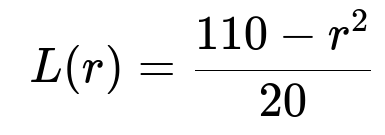
L(r) as the expected payoff if you guess that the blue ball’s value b is larger than r.
S(r) as the expected payoff if you guess that the blue ball’s value b is smaller than r.
It can be shown that:

A simple analysis reveals L(r) > S(r) for r from 1 up to 7, and L(r) < S(r) for r from 8 to 10. Thus, the optimal strategy is:
If r <= 7, guess that b is larger.
If r >= 8, guess that b is smaller.
Under this strategy, the expected payoff is 4.375 dollars. Because you have to pay $4.50 to play, the game is not fair; the house has an edge of about 2.8%.
Comprehensive Explanation
Payoff Structure and Notation
Each beaker (red and blue) contains balls numbered 1, 2, …, 10. One ball is drawn randomly from each beaker.
You observe r, the number from the red beaker. The number b from the blue beaker is unknown.
Your decision: guess “b > r” or “b < r.”
If you guess correctly which is larger, you receive b dollars.
If r = b, you receive (1/2)*b dollars.
If you guess incorrectly about which is larger, you get 0 dollars.
Because r is revealed to you, you can tailor your guess to maximize your expected gain for each possible value of r. Then you pay $4.50 to the house to participate.
Computing Expected Payoff Conditioned on r
The random variable b is uniformly distributed among {1, …, 10} but hidden from you.
For a given r, define L(r) = expected payoff if you guess b is larger.
Define S(r) = expected payoff if you guess b is smaller.
Deriving L(r)
If you guess b is larger than r:
The event b > r occurs with probability (# of blue-ball values strictly greater than r) / 10.
Whenever b > r, you gain b dollars.
The event b = r occurs with probability 1/10. In that case, you gain (1/2)*r.
The event b < r yields zero payoff.
Hence,
The sum of all possible b > r is the sum of the integers from r+1 to 10. This sum is ( (r+1) + 10 ) * (10 - r ) / 2 if you use the arithmetic series formula. Dividing by 10 (the total number of possible b values) gives the expected value from the b > r scenario.
Additionally, with probability 1/10, you earn (1/2)*r.
Carrying out the algebra leads to:
Deriving S(r)
If you guess b is smaller than r:
The event b < r occurs with probability (# of blue-ball values strictly less than r) / 10.
Whenever b < r, you gain b dollars.
If b = r, you gain (1/2)*b = (1/2)*r, but that is zero for “guess b < r” if you interpret strictly. However, in practice, if b = r, you were not correct about which is larger, so you only get (1/2)*r when you guess incorrectly about which is larger. But the puzzle states “If r = b, you receive (1/2)*b dollars,” so you do receive (1/2)*r in that scenario. Because your guess “b < r” is not strictly correct if r = b, it might seem contradictory. However, the puzzle clarifies you still get half. So effectively, the probability that b = r is 1/10, giving (1/2)*r payoff.
The event b > r yields zero payoff in this scenario.
By similar arithmetic for the sum of the integers from 1 up to r-1 (whenever r > 1), one obtains:

Finding the Optimal Strategy
To decide whether to guess “b > r” or “b < r,” you compare L(r) and S(r) for each r from 1 to 10.
For 1 <= r <= 7, we find L(r) > S(r).
For 8 <= r <= 10, we find L(r) < S(r).
Thus, the best strategy is:
If r <= 7, guess “b > r.”
If r >= 8, guess “b < r.”
In a continuous sense, one might set 110 - x^2 = x^2, solving for x in the reals. This gives x^2 = 55 => x = sqrt(55) ~ 7.4. Since r must be an integer, you choose r <= 7 to guess bigger, and r >= 8 to guess smaller.
Computing the Final Expected Payoff
Under this strategy, each r = 1 through 7 leads to expected payoff L(r), and each r = 8 through 10 leads to expected payoff S(r). Because r is uniformly distributed over {1, …, 10}, we average:
Expected payoff = ( (sum of L(r) for r=1..7) + (sum of S(r) for r=8..10) ) / 10
Numerically, that total is 4.375 dollars.
Subtracting the Game’s Cost
You pay $4.50 to play. Since your expected return is 4.375 dollars, your expected net is 4.375 - 4.50 = -0.125 dollars. Thus, on average, you lose 12.5 cents each time you play. The house edge is approximately 2.8% relative to the 4.50 cost of play.
Verification by Simulation
Below is a quick Python code snippet showing how to brute force the expected payoff:
import itertools

# We will simulate all r in [1..10] and b in [1..10].
# For each r, we guess "b > r" if r <= 7, else guess "b < r".

def payoff(r, b):
    # If guess "b > r"
    if r <= 7:
        if b > r:
            return b
        elif b == r:
            return b / 2.0
        else:
            return 0
    # If guess "b < r"
    else:
        if b < r:
            return b
        elif b == r:
            return b / 2.0
        else:
            return 0

# Average over all possible pairs (r, b)
total = 0
count = 0
for r in range(1, 11):
    for b in range(1, 11):
        total += payoff(r, b)
        count += 1

expected_value = total / count
print("Expected Payoff without cost = ", expected_value)

# Subtract the cost
print("Net after $4.50 cost = ", expected_value - 4.50)
If you run this code, you will obtain an expected payoff of 4.375, leading to a net -0.125 dollars after paying $4.50.
Potential Follow-up Question 1: How would the strategy change if the payoff for a correct guess was, say, 2*b instead of b?
In this modified game, whenever you guess correctly which is larger, you receive 2*b dollars. If r = b, presumably you would receive b dollars (assuming the same half rule). The definitions for L(r) and S(r) would change accordingly:
L(r) = (1/10) * sum over (b in {r+1..10}) of 2b + (1/10)(1/2)*(r) for b = r
S(r) = (1/10) * sum over (b in {1..r-1}) of 2b + (1/10)(1/2)*(r) for b = r
You would need to recalculate these sums and compare them. Because 2*b grows more quickly with b, the threshold r at which S(r) surpasses L(r) could shift. Typically, you’d expect to guess “b > r” for a slightly larger range of r values because the reward for a larger b is now doubled.
Potential Follow-up Question 2: What if the cost to play changed?
If the entry fee were, for example, $4.00 instead of $4.50, you would compare the same expected payoff of 4.375 dollars with the new cost of 4.00 dollars. In that scenario, your expected net would be +0.375 dollars, making it a profitable game for the player. The house’s advantage or disadvantage depends entirely on the difference between the cost and your expected payoff under the best strategy.
Potential Follow-up Question 3: How would this approach scale for more balls or for different distributions?
If each beaker had n distinct balls (numbered 1 through n), you would generalize your payoff functions L(r) and S(r) in exactly the same way. You would compute:
L(r) = Probability(b > r) * expected value of b given b > r + Probability(b = r) * (1/2)*r
S(r) = Probability(b < r) * expected value of b given b < r + Probability(b = r) * (1/2)*r
As n grows large, you might solve for the approximate boundary of r that equates L(r) and S(r). When the distribution is not uniform or when ball numbering follows a different scheme, you adapt the sums or integrals to reflect that new distribution. The fundamental method—comparing the two expected values—remains unchanged.
Below are additional follow-up questions
Additional Follow-up Question 1: What if the number of balls is unknown or not disclosed?
One realistic twist is that you might not know exactly how many balls are in the beaker, or perhaps you only know an upper bound. Without knowing the exact distribution of the blue ball b (or the exact range of its values), your strategy must rely on partial information and assumptions about the possible outcomes.
Possible Pitfalls:
If you underestimate the range of b, you might incorrectly assume it is unlikely to be much larger than r. Then you would guess “b < r” more often, potentially missing out on valuable payoffs when b is actually high.
If you overestimate the range of b, you might repeatedly guess “b > r” and thus lose whenever b is not actually above r.
The difference in the payoff formula (you receive b dollars only if you guess correctly) means you must carefully weigh risk vs. reward when the distribution is not fully known.
In-depth Rationale:
Without certainty about b’s distribution, you can only use prior or subjective probabilities. You might assume a uniform distribution over some range, or rely on a Bayesian update if partial clues are revealed. You might also consider the cost of the game vs. potential payoffs.
A robust approach is to define an expected payoff model E[b] conditioned on each r, and compare your guess outcomes in a manner similar to the known case, but with bounds replaced by your assumptions about the likely range of b.
In an interview context, demonstrating an ability to handle incomplete information is critical: you must acknowledge the need for assumptions, sensitivity analyses (how your expected payoff changes if your distributional assumptions shift), and scenario testing for different possible ranges of b.
Additional Follow-up Question 2: What if you are allowed to switch your guess after seeing partial information about b?
Suppose you make an initial guess but then the carnival master gives you some hint about b (for instance, that b is even or that b is in the top half of its range), after which you can choose to stick to your guess or switch.
Potential Pitfalls:
A partial clue might lead you to misinterpret probabilities. For example, if you learn b is even, that changes the set of possible b values. You must recalculate the conditional expectation using only even b values.
If you fail to recognize that your initial guess might no longer be optimal given the new clue, you could make suboptimal decisions.
Detailed Logic:
For each possible r, you initially decide “b > r” or “b < r.”
After a hint, you update the distribution of b. For example, if b is even, the sample space of b is {2, 4, 6, 8, 10}. You would then re-compute your expected payoff of staying with the same guess vs. switching.
The game becomes more nuanced because you need to factor in the probabilities of receiving each type of hint, as well as how the hint changes the probabilities that b > r or b < r. In a practical scenario, you would need a systematic approach to evaluate new partial information.
Additional Follow-up Question 3: How does the strategy change if the carnival master can choose which r to reveal rather than drawing at random?
If the carnival master is not drawing r randomly but instead can choose which r to reveal, and you do not know that r was chosen strategically (or how it was chosen), the game changes drastically.
Key Implications:
The carnival master might exploit your known strategy. For instance, if your strategy is: “Guess b > r for r <= 7; guess b < r for r >= 8,” the carnival master might only offer r = 7 or r = 8 under circumstances that favor the house.
Your expected payoff might be lower than the calculated 4.375 dollars, because you assumed r was equally likely to be any integer from 1 through 10.
In-depth Analysis:
If the carnival master can choose r to maximize your losses, they might pick an r that gives them the largest house edge. For instance, maybe they pick r = 7 when b is actually not bigger or pick r = 8 when b is actually bigger.
To analyze this scenario, you would shift from assuming uniform distribution of r to a worst-case distribution. You would attempt to find a minimax strategy that maximizes your payoff under the worst possible choice of r.
This is akin to a game theory problem: you have your decision rule, the carnival master has a counter-strategy, and the equilibrium might be different than the straightforward solution that assumes r is random.
Additional Follow-up Question 4: What happens if the payoff for a correct guess is not linear in b?
Consider a variant where your payoff is f(b) for some function f(b) (e.g., sqrt(b), log(b), b^2, etc.), still receiving half of that if b = r.
Pitfalls & Edge Cases:
Nonlinear functions can shift the relative advantage of guessing “larger” vs. “smaller.” For instance, if the function grows very quickly (like b^2), then the potential reward for guessing that b is larger might dominate unless r is extremely high. Conversely, if the function grows very slowly (like log(b)), the difference between guessing high or low might be less pronounced.
If f(b) takes on negative values under certain conditions (unlikely but possible in a contrived setting), you would need to consider the risk of negative payoffs.
Detailed Explanation:
The new L(r) and S(r) become integrals or sums of f(b) over the relevant subsets of b. For example, L(r) = (1/10) * sum_{b=r+1..10} f(b) + (1/10)*(1/2)*f(r).
You compare L(r) and S(r) for each r to find the threshold at which they are equal. Solve f-based equations accordingly.
In an interview, you should outline how to set up these sums, handle the half-payoff in the r = b case, and re-derive the threshold to demonstrate your mathematical and problem-solving skills.
Additional Follow-up Question 5: How do you handle repeated plays with a limited bankroll?
If the game allows repeated attempts, but you must manage a limited capital, you have to factor in risk management. Even if the expected value might be slightly negative or positive, your bankroll can be wiped out by bad runs.
Detailed Considerations:
Kelly Criterion: In betting scenarios, one approach is to size each bet proportionally to your advantage (if any) to avoid ruin. However, in this carnival game structure, there is a fixed cost per play of $4.50, so you do not have the option of “betting less.” You either pay the entire entry fee or do not play at all.
Variance and Probability of Ruin: The game’s payoff might have high variance because b can range from 1 to 10, and your net outcome can vary from 0 to 10 in each round (minus 4.50). Over multiple plays, you risk a streak of unfortunate guesses or unlucky draws.
Interview Insight: If asked, you should mention that repeated plays require a broader portfolio approach to risk management. Even a slightly negative expected value game can be played if you have other offsetting strategies that yield positive expected values overall. In practical gambling or real-life scenarios, you weigh the net effect on your total capital.
Additional Follow-up Question 6: Could psychological or behavioral factors affect the decision-making process?
Though the mathematically optimal strategy is clear, in real life, players might deviate from purely rational decisions.
Common Behavioral Traps:
Loss Aversion: After a few rounds of losing, a player might chase losses by changing strategy. For instance, if they keep losing with r = 7 by guessing “b > r,” they might psychologically be tempted to switch to “b < r,” even though the mathematical advantage is still in “b > r.”
Overconfidence: If a player experiences a lucky streak, they might guess “b > r” too frequently, ignoring the times when r is already large.
Anchoring: Because r is visible, a player might anchor on that number without re-evaluating the distribution of b thoroughly.
Deep Explanation:
Behavioral economics research shows that even when the expected value is in front of them, people tend to misjudge probabilities (e.g., the gambler’s fallacy). Interviewers might probe whether you understand these human factors, especially if you are designing machine learning models for real-world decisions where human bias is relevant.
If you create an AI agent to play this game, it would not suffer these biases, and it would execute the optimal strategy systematically. However, in practice, the carnival relies partly on human irrationality to ensure a house edge.