
ML Interview Q Series: Central Limit Theorem: Normality from Averages and Its Importance for Machine Learning Inference.
📚 Browse the full ML Interview series here.
Central Limit Theorem: Explain the Central Limit Theorem and why it is important in machine learning. For example, if you take the average of 100 independent random variables, how does the distribution of that average relate to the distribution of the individual variables, and how can this be useful in practice?
Understanding the core idea of the Central Limit Theorem (CLT) and its importance in machine learning hinges on grasping how the distribution of sums or averages of independent random variables behaves, especially as the sample size grows. It is one of the most important results in probability theory and underpins a great deal of inferential statistics and confidence-estimation techniques commonly applied in machine learning workflows.
The theorem states that if you have a set of independent and identically distributed (i.i.d.) random variables with a given mean and variance, then as you increase the number of these random variables that you sum (or take the average of), the resulting distribution of that sum (or average) approaches a normal distribution. This is true regardless of the original distribution, provided the original distribution has finite mean and variance.
Why this matters in machine learning is that many practical tasks rely on averaging, aggregating, or drawing inferences from data samples. Even if individual data points come from unknown or non-normal distributions, the sample mean often ends up having an approximately normal shape once you have a sufficiently large sample size. This gives machine learning practitioners a stable foundation for constructing confidence intervals, hypothesis tests, and for understanding how errors or estimates may be distributed.
Use cases in practice often involve model evaluation and error estimation: for example, if one calculates the average error across multiple batches, the CLT helps justify why standard error bars around that mean error might be modeled using normal distributions.
Relation of the distribution of an average of 100 i.i.d. variables to the distribution of individual variables can be summarized as follows: even if the original variables have a strongly skewed or heavy-tailed distribution (provided it has finite mean and variance), the distribution of their sample mean converges to a normal distribution as the sample size increases. With 100 independent samples, the approximation might already be decently close to normal, depending on the shape of the original distribution.
Detailed explanation of the core concept can be understood through a simple mathematical expression for the sum or mean of i.i.d. random variables, although we will only present it in a minimal form here for clarity:
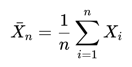
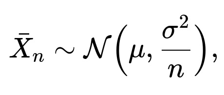
where each (X_i) is an i.i.d. random variable with mean (\mu) and variance (\sigma^2). The Central Limit Theorem states that if (n) is large, then:
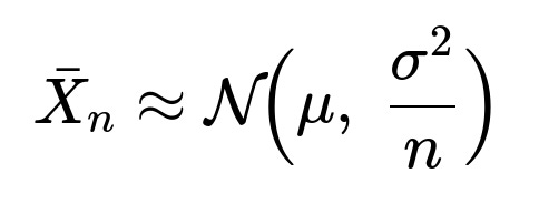
In other words, (\bar{X}_n) is approximately normally distributed with mean (\mu) and variance (\sigma^2 / n). When used in practice, this implies:
The distribution of (\bar{X}_n) is much more “bell-shaped” and concentrated around the true mean (\mu) compared to the distribution of any single one of the (X_i).
Standard error of the mean (which is proportional to (\sigma / \sqrt{n})) shrinks as (n) grows.
In a machine learning context, whether you are estimating a validation accuracy, a mean squared error across multiple runs, or constructing confidence intervals for your model’s performance, the CLT gives a theoretical basis that the average of many observations is approximately normal. This simplifies both computation and interpretation of confidence intervals (like using Z-scores or t-distributions for smaller (n)).
Practical example in code might look like this:
import numpy as np
import matplotlib.pyplot as plt

# Generate a non-normal distribution, e.g., exponential
np.random.seed(42)
num_samples = 100000
x = np.random.exponential(scale=1.0, size=num_samples)

# Now compute the average of smaller chunks (groups of size 100)
chunk_size = 100
chunks = num_samples // chunk_size
averages = []
for i in range(chunks):
    sample_chunk = x[i*chunk_size : (i+1)*chunk_size]
    averages.append(np.mean(sample_chunk))

# Plot histogram of the original distribution vs the distribution of averages
plt.figure(figsize=(12,5))
plt.subplot(1,2,1)
plt.hist(x, bins=50, density=True, alpha=0.7, color='blue')
plt.title("Original Exponential Distribution")

plt.subplot(1,2,2)
plt.hist(averages, bins=50, density=True, alpha=0.7, color='green')
plt.title("Distribution of Averages of 100 samples")

plt.show()
In the left histogram, you see the heavy right skew of the exponential distribution. In the right histogram, you see that the distribution of the averages of groups of size 100 is visually much closer to a bell shape, illustrating the CLT in practice.
This result is extremely useful because it holds even when the original distribution is unknown, as long as the fundamental conditions (like independence and finite mean/variance) are satisfied. Moreover, it provides a simpler way to characterize the distribution of an estimator’s mean or total sum. It is the theoretical underpinning for many common statistical procedures that machine learning practitioners rely on for diagnosing model performance, constructing intervals for uncertainty, and more.
What are some common pitfalls or subtlety to watch out for?
One of the key assumptions is that the random variables must be at least approximately independent and identically distributed and have finite variance. If there is significant correlation or the variance is infinite, the CLT in its simplest form may fail to apply or might give misleading results. In real-world scenarios, data can sometimes be correlated (like time series data in machine learning problems). Variants and extensions of the theorem for dependent data do exist (for example, the mixing conditions used in time-series analysis), but one must be careful.
Another subtlety involves the rate of convergence. For distributions that are heavy-tailed or heavily skewed, you might need a large (n) to get a good approximation. A typical “rule of thumb” is that you need 30 or more samples to start seeing a shape that’s “normal enough,” but that depends heavily on the underlying distribution.
How is it useful in practice?
It is fundamental to forming confidence intervals in many real scenarios. For example, when we estimate a model’s accuracy by sampling multiple datasets or by doing cross-validation, we often compute the mean accuracy across folds and then place confidence intervals around that mean. We rely on the assumption that this mean follows a normal distribution for large (n), letting us say things like “the 95% confidence interval is the sample mean ± 1.96 times the standard error.” This is a direct application of the CLT.
It also appears in the context of gradient estimates in stochastic gradient descent. Although not always framed explicitly in terms of the CLT, the principle that averages of independent gradient estimates approximate the true gradient in a normal-like manner is highly relevant in analyzing the variance of gradient-based optimization steps.
Common Interview Follow-up Questions
What if the random variables are not independent or not identically distributed?
One must recall that the standard (classical) Central Limit Theorem assumes i.i.d. data. There are variations, such as the Lindeberg, Lyapunov, or other generalized central limit theorems, that relax the requirements slightly. In a machine learning setting, data can be correlated in time (like a time series) or space (like images in a video). When these correlations are strong, the naive CLT might break down or converge more slowly, and you’d need to apply a version of the CLT that accounts for dependencies. Many real-world processes have short-range dependencies or “weak dependence,” and those processes still have versions of the CLT that apply under certain mixing conditions. However, for a highly structured correlation (like some complicated dynamic system), the normal approximation could be inaccurate.
How does the distribution of the sum (as opposed to the mean) behave under the Central Limit Theorem?
The difference between the sum and the mean is just a factor of (1/n). For large (n), summing (n) i.i.d. random variables produces a distribution whose mean is (n\mu) and variance (n\sigma^2). By normalizing that sum by (n), you get the average, which has mean (\mu) and variance (\sigma^2/n). Both the sum and the mean, after a suitable normalization (subtracting the mean and dividing by standard deviation), tend to a standard normal distribution. This is precisely why many statements of the CLT focus on the sum (\sum X_i), then extend it to the average (\bar{X}_n).
Why do we typically assume independence in the CLT, and is it an absolute must?
Independence is one of the simplest ways to ensure that the variables do not carry overlapping information that might break or slow down the convergence to normality. If variables are correlated, the effective sample size might be smaller than (n), and more complicated assumptions are required to ensure you still get a normal approximation. Weak correlation can sometimes be handled, but strong correlation across variables means you might need a different theoretical tool or a different version of the CLT that allows for correlated data. In practice, many large datasets behave “as if” samples are nearly independent, especially if the sampling is done randomly across a diverse population. But it is crucial in time-series or spatial data to check how strong those correlations are.
How does the CLT apply to practical model evaluation in machine learning?
In evaluating models, people often run repeated experiments or perform cross-validation to get an aggregate performance metric (like average accuracy or average loss). Due to the CLT, these averages typically end up looking approximately normal. This lets you place standard confidence intervals around an accuracy estimate or around a difference in performance between two models. Even though the underlying distribution of each individual accuracy measurement might not be normal (accuracy is often bounded between 0 and 1, and each experiment might be subject to different random seeds, slight data variations, etc.), the average of a large enough set of experiments tends to a normal shape. That normal approximation becomes the basis for t-tests, Z-tests, or constructing simpler standard error bars on your model accuracy chart.
What if the underlying distribution has infinite variance?
A crucial requirement for the classical CLT is that each (X_i) has finite variance. If the variance is infinite, such as with certain heavy-tailed distributions (for instance, some stable distributions like Lévy or Pareto distributions in certain parameter regimes), the CLT in its usual form does not hold. In such cases, the sum or average may follow a stable law that does not converge to a Gaussian, and standard methods relying on the normal approximation may fail badly. In ML tasks where data can have heavy tails (e.g., extremely large but rare outliers in real-world data), you must ensure that you either mitigate the outliers or use robust techniques that do not rely purely on the classical CLT assumption.
How do we estimate how many samples we need for a “good” normal approximation via the CLT?
There is no universal fixed rule. Some rule-of-thumb guidelines say 30 to 50 samples is enough to see the bell shape emerging if the underlying distribution is not too skewed or heavy-tailed. But in practice, you judge convergence by visually inspecting histograms or applying normality tests (like the Shapiro-Wilk test) on your sample averages. If your data distribution is extremely skewed or has heavy tails, you might need hundreds or thousands of samples before the mean distribution looks Gaussian. In the context of big data scenarios in machine learning, once you have a large dataset or many repeated experiments, the mean’s distribution often reliably appears normal.
How do we incorporate the CLT into hyperparameter tuning or cross-validation setups?
When performing cross-validation for hyperparameter tuning, you might measure the performance (like validation loss or accuracy) across multiple folds. Each fold represents a random subset of the data. By collecting the mean performance across those folds, you can approximate how well the hyperparameter setting performs on average. Thanks to the CLT, you can treat that average as approximately normal, which lets you compute confidence intervals or do significance tests between different hyperparameter choices. Although the independence assumption can be fuzzy—folds may partially overlap—the approximation is frequently good enough to guide practical decisions in ML development pipelines.
How does the CLT relate to the Law of Large Numbers (LLN)?
The Law of Large Numbers (LLN) states that (\bar{X}_n) converges to the true mean (\mu) almost surely (Strong LLN) or in probability (Weak LLN) as (n \to \infty). That addresses convergence in terms of the value of (\bar{X}_n). The CLT, by contrast, describes the distribution around that mean as (n) grows. The CLT gives a richer view: not only does the sample mean converge to (\mu), but any deviations from (\mu) become normally distributed around (\mu) with variance shrinking like (1/n). Thus, the CLT gives us the rate and shape of convergence, while LLN just says convergence happens but does not specify the shape around (\mu).
How can we leverage the CLT for variance reduction in Monte Carlo methods?
A direct application of the CLT appears in Monte Carlo simulations, where one estimates an expected value by averaging many random samples. The CLT tells us that each estimate’s distribution narrows around the true mean as we increase the sample size. It also implies that if we can reduce the variance of each sample (for example, through control variates, importance sampling, or other variance-reduction techniques), then we more quickly arrive at a stable estimate. Being able to say “the distribution of your average is normal with this variance” makes it straightforward to place error bars on Monte Carlo estimates, crucial in simulation-based approaches used in certain machine learning tasks and Bayesian inference contexts.
How to think about the CLT from a high-level perspective in data science or ML interviews?
Often, the key takeaway is that the CLT justifies using normal distributions as a go-to assumption for aggregated statistics, even when the original data is not normal. It is the reason standard test statistics, confidence intervals, p-values, etc., have widespread usage. Understanding the core assumptions (independence, identical distribution, finite mean/variance) and their pitfalls in real-world scenarios is critical for advanced roles. Engineers who know how to detect violations of these assumptions and adjust or adopt robust methods or alternative theorems (like the Delta Method or generalized CLT variants) are better equipped to handle complex data challenges.
Additional Follow-up Questions and Answers in More Depth
Are there special cases where the CLT does not help?
If data is fundamentally discrete with only a few possible outcomes (e.g., Bernoulli variables), the CLT still applies, but for very small (n) you might see a distribution that is not at all bell-shaped. For example, the distribution of the sum of Bernoulli(0.5) random variables for small (n) looks binomial, which can be significantly skewed when (n) is not large. As (n) increases, it does become approximately normal. But if you only have tiny sample sizes, referencing the CLT might not give an accurate picture, and you might prefer exact binomial confidence intervals.
How does the CLT help in building confidence intervals for model error?
Confidence intervals for a model’s prediction error can be formed if you can assume that your error terms are i.i.d. with finite variance. By sampling your model’s predictions or by using cross-validation splits, you collect multiple measurements of error. You then compute the mean error and its standard deviation. Because of the CLT, you assume the average error is normally distributed for large sample sizes:
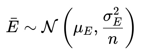
Hence, you get:
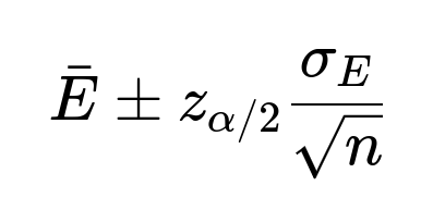
where (z_{\alpha/2}) is the critical value (for a 95% confidence interval, (z_{0.025} \approx 1.96)). This is a direct and common usage in ML for explaining how certain you are about your performance metric.
How do we handle small-sample scenarios if we still want to use normal approximations?
For small (n), the t-distribution is often used instead of the Z-distribution. The t-distribution is a heavier-tailed distribution that better accounts for the additional uncertainty you have in your estimate of (\sigma). The t-distribution converges to the standard normal distribution as (n) gets larger, which also aligns with the CLT perspective that with sufficient data, your mean is well-approximated by a normal distribution.
Why is the Central Limit Theorem so frequently mentioned in Data Science and Machine Learning interviews?
Because it is foundational for understanding why “averages” often show normal-like behavior in real-world data scenarios. It is also fundamental to core statistical tasks such as computing confidence intervals, hypothesis testing, and error bars for model metrics. In addition, advanced topics like approximate Bayesian computation or large-scale MCMC can rely on the normal approximation of aggregates or means. Knowing when it applies, when it fails, and how to adapt is viewed as a litmus test for a candidate’s depth in machine learning and statistics.
How would you quickly explain the CLT to someone with minimal background?
You could say: “If you keep taking averages of random draws from the same source, the result of those averages will follow a bell-shaped curve, no matter what the initial shape of the source distribution was, provided the source has a finite average and variance. The more draws you average, the tighter that bell gets around the true average.” In a job interview, elaborating on i.i.d. assumptions and acknowledging real-world complexities is essential to demonstrate practical awareness.
Are there any robust checks we can run to see if the CLT-based assumptions in our ML experiments are valid?
One might generate a Q-Q plot (quantile-quantile plot) of your sample means or errors against a theoretical normal distribution. If the points lie roughly on a straight line, it suggests the distribution is close to normal. Another check is to use normality tests, though they can sometimes be sensitive to large sample sizes (they might detect “tiny” deviations from normal that are not practically relevant). Overall, visual inspection plus domain knowledge about your data’s correlation structures, outliers, or distribution shape can guide you as to whether the CLT is being applied appropriately.
How can knowledge of the CLT help with interpretability of ensemble methods in ML?
In ensemble learning, you combine predictions from multiple base models. If you see that each base model’s prediction is an i.i.d. random variable (not strictly i.i.d., but often we assume they are “fairly independent” in some sense), then the CLT might suggest that the average prediction across these models is more stable (less variant) and might exhibit approximately normal fluctuations around the true target. This perspective can help in analyzing and understanding why ensemble methods often yield better and more stable performance than individual models. It also supports building confidence bands around ensemble predictions in certain conditions.
When the ensemble models are highly correlated, the effective independence is decreased, so you get less variance reduction from averaging than the CLT’s naive form might suggest. That ties back into the importance of independent assumptions in the CLT.
How do we explain the “speed” of convergence to a normal distribution in the CLT?
This is related to Berry-Esseen bounds and other refined theorems that quantify how quickly the distribution of (\bar{X}_n) converges to a normal distribution. They provide bounds on the difference between the actual distribution and the limiting normal distribution, usually in terms of the third central moment (skewness) of the underlying distribution. The simpler version is that the rate of convergence is on the order of (1/\sqrt{n}). Practitioners typically do not compute these exact bounds in day-to-day ML, but it is good to be aware that if the distribution is extremely skewed, you might need a larger (n) to achieve the same “closeness to normal.”
Why does the CLT not require that the random variables come from a normal distribution themselves?
This is precisely the remarkable aspect of the CLT: it demonstrates a form of universality. The distribution can be exponential, binomial, Bernoulli, uniform, or any other distribution with finite variance, yet the sample mean eventually yields a bell-curve shape when (n) becomes large. This universality is a profound insight—why so many real-world phenomena lead to normal-like distributions (e.g., sums of many small independent effects). In machine learning, data often arises from highly complex or unknown distributions, but this theorem suggests we can often rely on normal-based approximations for aggregated statistics.
Could you give an intuitive explanation for the “why” behind the CLT?
An intuitive explanation is to think about how each random draw adds small “random shocks” to the total sum. If these shocks are independent, then sometimes you get a positive “push,” sometimes negative, and these increments tend to cancel each other out over large numbers. Once you have many such increments, the distribution of their sum (or average) is dominated not by the peculiarities of one shock but by the collective effect. The math of the CLT shows that this collective effect leads to a Gaussian pattern, because the Gaussian distribution is the fixed point under repeated convolution of distributions with finite variance. This also connects to the idea that the Gaussian is the “maximum entropy distribution” for a given mean and variance, which is a related but slightly different perspective from the classical CLT statement.
When do I need to be cautious applying the CLT in ML contexts?
Any time your data is not i.i.d., or you suspect infinite-variance phenomena (e.g., extremely heavy-tailed distributions), or you only have a small sample size. If your sample size is small, you can’t rely heavily on the normal approximation (though you can pivot to t-distributions if the data is still reasonably well-behaved). If your data is heavily correlated, you may be effectively averaging fewer “independent” pieces of information than you think. Also, if you have intense outliers that might distort the sample mean, the variance might not be well-defined (or be inflated by outliers). In such scenarios, robust statistics or transformations might help bring the data to a form more amenable to the CLT assumptions.
Summary of Why the CLT is Important in Machine Learning
It is a cornerstone of inferential statistics, enabling normal approximations for means of random variables even if each variable is drawn from a non-normal distribution. Machine learning often involves computing performance metrics by averaging errors or accuracies, or combining gradient estimates. The CLT provides the theoretical basis for constructing error bars, confidence intervals, and for understanding the stability of ensemble methods. Despite its simple statement, it is foundational for the rigorous application of many statistical and analytical tools in the ML pipeline, from experiment design and result interpretation to advanced ensemble methods and large-scale simulations.
Additional Practical Example: Confidence Intervals in Validation Metrics
One direct application is in building confidence intervals for a classification accuracy metric. Suppose you have performed multiple runs of a model on slightly different train-validation splits. Let (X_1, X_2, \dots, X_n) be the observed accuracies. If each run is an approximately independent draw from the same distribution of possible model performance (which is a bit idealized, but let’s assume so for simplicity), you can apply:
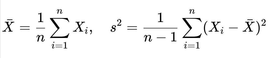
The standard error of the mean is approximately (s / \sqrt{n}). By the CLT, (\bar{X}) is approximately normal, so a 95% confidence interval for your model’s average accuracy is:
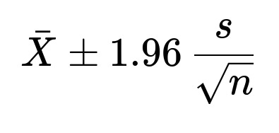
(because 1.96 is the z-score for 95% coverage under a standard normal distribution). This formula is widely used in academic papers, Kaggle competitions, and real-world model reporting to communicate how stable or variable the model’s performance might be across different data splits.
Below are additional follow-up questions
How does the CLT handle continuous vs. discrete distributions, and are there any practical differences in convergence behavior?
When applying the Central Limit Theorem (CLT), the key assumptions (independence, identical distribution, finite variance) hold for both discrete and continuous random variables. In practice, the theorem’s statement that sums or averages of such variables converge in distribution to a normal distribution remains the same. The difference is not in how the CLT is stated, but in how quickly the convergence occurs and how easily you can check the i.i.d. conditions in real data.
One potential subtlety is that for discrete random variables with only a few possible outcomes (e.g., Bernoulli or other low-support categorical distributions), the shape of the distribution of sums might be distinctly non-normal for smaller sample sizes. For instance, a binomial distribution can be highly skewed if the probability of “success” is very low or very high. As your sample size grows, the CLT still holds, but you might need more samples to see a bell curve emerge.
Pitfalls arise when you have discrete data that violate independence. Real-world classification tasks, for example, can produce discrete predictions that might be correlated in time or correlated via the environment in which they were sampled. These correlations can slow the convergence to a normal distribution. Additionally, finite variance must hold in both discrete and continuous cases. Some discrete distributions with heavy tails (such as certain power-law distributions over integer support) can have infinite variance, which invalidates the classical CLT.
What is the characteristic function approach to the CLT, and how might it be used in machine learning?
A characteristic function of a random variable (X) is the expected value of (e^{itX}), often denoted (\phi_X(t)). It captures all moments of the distribution (if they exist) in the frequency domain. The proof of the CLT using characteristic functions is often taught in advanced probability courses. It shows that when you look at the characteristic function of a sum of i.i.d. random variables, it converges pointwise to the characteristic function of the normal distribution as the number of terms grows.
In machine learning, the characteristic function approach can be instructive if you need deeper insights into how sums of random variables transform under certain constraints (for example, in Fourier-based methods or signal processing contexts). It is also relevant in some Bayesian or MCMC methods where you want to formally prove that your estimates converge to a certain distribution, and characteristic functions can provide a powerful way to establish these convergence properties.
A subtlety arises when data is heavily correlated or lacks finite variance. In that scenario, analyzing the characteristic function becomes more complex—some random variables (especially heavy-tailed) do not have well-defined characteristic function expansions beyond certain orders. Moreover, in real-world ML tasks, explicit characteristic function analysis might be overkill unless you are dealing with specialized inference methods that rely on transformations in the frequency domain.
Could you elaborate on the Berry–Esseen theorem and how it refines the CLT in practical applications?
The Berry–Esseen theorem provides bounds on the rate at which the distribution of the normalized sum (or mean) of i.i.d. random variables converges to the standard normal distribution. Specifically, it quantifies the maximum distance between the cumulative distribution function (CDF) of the scaled sum and the CDF of a standard normal distribution. It does this in terms of the third absolute moment (essentially the skewness-related term) of the underlying random variables.
In practice, this means that if you want to know how large (n) needs to be for a “good enough” approximation by the normal distribution, Berry–Esseen gives a more concrete answer than the classical CLT alone. It provides an inequality of the form:
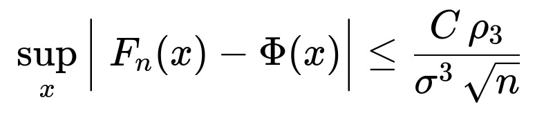
Here, (F_n) is the CDF of your normalized sum, (\Phi) is the standard normal CDF, (\rho_3) is the third absolute moment about the mean, (\sigma^2) is the variance, and (C) is a constant (often cited as 0.4784, though exact values can vary in references).
The subtlety for machine learning arises when dealing with non-stationary or skewed data. If (\rho_3) is large—implying a heavily skewed or long-tailed distribution—the bound might say you need many more samples to achieve the same closeness to the normal approximation. Also, Berry–Esseen typically addresses i.i.d. data; if you have correlated or heteroskedastic data, the bounding approach needs extensions or modifications.
How might the CLT be applied or adapted for real-time streaming data where the underlying distribution could shift over time?
In real-time streaming scenarios, one often uses running averages, exponential moving averages, or rolling windows to maintain estimates of means and variances on the fly. The CLT conceptually still applies if data chunks are somewhat i.i.d. or at least stationary over short intervals. For a large enough window, the average can be approximated by a normal distribution, and you can build confidence intervals around that estimate.
A critical pitfall is distribution shift—if the data’s mean or variance changes over time (concept drift in streaming contexts), the CLT-based confidence intervals or normal approximations might become stale. In other words, the old data no longer has the same distribution as the new data. This can lead to misleading intervals or hypothesis tests unless you adapt your window size or weigh recent data more heavily.
In real-time ML applications such as anomaly detection or online learning, you often assume “weak stationarity” or attempt to detect changes in distribution. Once a shift is detected, you might reset your accumulation of sums, re-initialize your statistics, or use an approach that adjusts quickly (like forgetting factors). Even then, strictly speaking, the classical CLT does not hold for data with abrupt or continuous shifts—extensions that allow for slowly changing distributions exist but have more complicated conditions.
How do conditions like Lindeberg’s condition or Lyapunov’s condition extend the CLT to non-identical distributions, and is this relevant in ML?
The Lindeberg and Lyapunov conditions are generalized criteria under which the CLT holds even if the random variables are not strictly identical in distribution. They require, broadly, that no single random variable in the sequence dominates the sum and that the variance of the sum grows sufficiently. If these conditions are satisfied, you can still get a normal limit for properly normalized sums.
In machine learning, data can come from slightly different distributions, especially if collected from diverse sources or at different times. If the data from each source or time slice has roughly the same scale and does not produce outliers that dominate the sum, then Lindeberg or Lyapunov conditions might apply.
A subtlety is that while these conditions are more general, they still require independence (or at least something close to it). If the variables are heavily correlated or have infinite variance, they won’t help. Another real-world challenge is verifying these conditions: it can be non-trivial to prove that no single random variable is too large relative to the sum. In practice, data scientists rely more on empirical checks—like looking for outliers or computing incremental statistics—rather than a formal Lindeberg check. Still, it is conceptually useful to know that the CLT can hold under weaker assumptions than i.i.d.
How does the CLT fare in adversarial or security-focused ML settings where data may not be purely random?
In adversarial ML scenarios, an attacker might inject data points designed to manipulate the model or the distribution of inputs. This disrupts the assumptions of independence or identical distribution. Because the CLT fundamentally relies on the premise that the underlying samples come from a stable, well-defined probability distribution with finite variance, adversarial data can artificially alter means, inflate variances, or create “poison” samples.
A direct result is that the normal approximation for your average or sums might be systematically biased or might underestimate variance. For example, a few carefully placed outliers could heavily shift the mean. In extremely adversarial contexts, we can’t rely on the CLT for robust confidence intervals. Instead, robust statistics or defenses that either remove or down-weight suspicious samples are needed. Some robust variants of the CLT assume that only a small fraction of samples are corrupted, but they typically require a form of “clean majority” assumption.
In distributed machine learning, how can the CLT be leveraged to combine partial statistics from different nodes, and what factors might interfere with its validity?
In distributed ML, multiple nodes might each compute partial means and variances of local data, then communicate those statistics to a central server. The central server can combine them to get an overall mean and variance. Because the sum (or weighted sum) of locally averaged values is just an aggregate of many i.i.d. samples (assuming each node’s data is representative of the same distribution), one can invoke the CLT to argue that this global average will be normally distributed around the true mean. This is often used to justify performing parameter averaging in distributed training or to maintain confidence intervals on aggregated metrics.
Subtleties arise when:
Different nodes see data that are not from the same distribution. One node might have data from a different population, or the data might shift over time on certain nodes.
The nodes are using different random seeds or different augmentation strategies, leading to correlations in the processed data.
Communication delays or asynchronous updates lead to “stale” statistics that do not align well in time.
Any of these issues can degrade the i.i.d. assumption, potentially slowing or invalidating the normal convergence. In practice, frameworks often assume approximate i.i.d. data partitioning to keep the analysis simpler. If distributions differ significantly (federated learning across heterogeneous devices, for instance), advanced methods or weighting strategies might be needed.
What are some ways the CLT can be used in approximate Bayesian computation, and what pitfalls might arise?
In approximate Bayesian computation (ABC) or in posterior approximation methods (like variational inference or certain Monte Carlo techniques), you often rely on sample-based estimates of likelihoods or posterior distributions. The CLT suggests that if you draw enough samples of a parameter or a likelihood from a stable process, the mean estimate (or the sum’s distribution) becomes approximately normal. This can simplify the approximation of posterior distributions around a mode or mean.
A pitfall is that posterior distributions can be multi-modal or strongly skewed in real-world Bayesian ML tasks. In that scenario, focusing on a single approximate normal near the mean might miss critical structures in the posterior. Furthermore, sampling in high-dimensional parameter spaces can slow the rate of CLT convergence, especially if there are correlations among dimensions. Techniques like Hamiltonian Monte Carlo or importance sampling might help, but the independence or stationarity assumptions are not trivially satisfied in MCMC chains with strong autocorrelation. The CLT still applies to ergodic Markov chains under certain mixing conditions, but verifying or ensuring sufficient mixing can be tricky.
How does the Delta Method extend from the CLT, and what are its real-world applications in ML metrics?
The Delta Method says that if you have a random variable ( \bar{X}_n ) that converges to a normal distribution (by the CLT, say), then a smooth function ( g(\bar{X}_n) ) also has an approximately normal distribution around ( g(\mu) ) for large (n). More formally, if
then for a differentiable function (g),
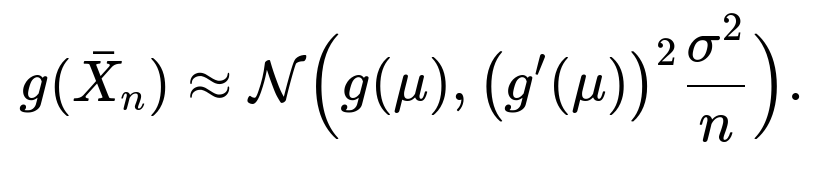
This is incredibly useful in machine learning when you want to approximate the distribution of a transformed statistic. For example, if your model performance metric is a function of the mean accuracy—maybe a log-odds transform or some more complex function—knowing the approximate distribution helps you construct confidence intervals or do hypothesis tests around that function of the mean.
A subtlety is that the function (g) must be smooth and differentiable around (\mu). If (g) has a discontinuity or a very flat region around (\mu), the linear approximation might be poor, causing the normal approximation to fail. Also, if your sample size is not large, or if (\bar{X}_n) has not stabilized (due to correlation or distribution shifts), the Delta Method’s approximation may be unreliable.
Are there specialized forms of the CLT for variables confined to the interval [0, 1], such as in classification probabilities?
For random variables strictly in [0, 1] (e.g., Bernoulli or Beta-distributed variables), there is still a classical CLT application if they are i.i.d. with finite variance. Their sums and averages will converge to a normal distribution, but the speed of convergence can be impacted by how close the distribution is to 0 or 1. If the true mean is near 0 or near 1, the distribution of sums can initially be quite skewed.
In classification tasks, each data point is typically a success/failure outcome (0 or 1). If the true probability is p, the sum of n Bernoulli trials has variance ( n p (1-p) ), which can be quite small if p is near 0 or 1, slowing the ratio of variance to n in a way that can lead to visible skew for smaller n. However, once n is large, you still get a normal approximation. A subtlety arises in highly imbalanced classification, where p might be extremely small or extremely large—then you might need many more samples to see a decent normal shape, or you might rely on exact methods (binomial confidence intervals) for smaller n.
How do hierarchical or multi-level structures in data complicate direct applications of the CLT?
In hierarchical or multi-level data, observations are grouped into higher-level units—like students within classrooms, or clients within regions. Often, within a group, samples are correlated, and the i.i.d. assumption is not valid across the entire dataset. The simplest form of the CLT no longer strictly applies because independence is violated.
Extensions like cluster-robust standard errors or random-effects models attempt to handle these correlations by modeling the data’s hierarchical structure. You might use specialized versions of the CLT that apply to “clustered data” under certain mixing or exchangeability assumptions. Real-world pitfalls include incorrectly assuming that all data points are i.i.d. when there is a clear group structure. This can lead to overconfident intervals or incorrectly sized hypothesis tests (e.g., you think you have more independent pieces of information than you actually do). In ML practice, ignoring hierarchy or correlation can yield overly optimistic performance estimates.
Can we rely on the CLT in non-parametric bootstrap methods without strong parametric assumptions?
Non-parametric bootstrap methods resample data from an observed dataset to approximate the variability of a statistic. The theory behind the bootstrap relies, in part, on CLT-like properties: if the original sample is representative of the population, then the distribution of the resampled statistic approximates the “true” distribution. As the sample size grows large, the resampled statistics tend toward a normal distribution around the true parameter.
One subtlety is that in a real-world setting, the bootstrap will be reliable only if the observed sample is a reasonable proxy for the entire population distribution. If the sample is biased or too small, the bootstrap might not approximate the distribution well. Further, the CLT’s independence assumption can be undermined by correlated data, meaning naive bootstrap resampling might not capture the correlation structure. Special block bootstrap or stationary bootstrap procedures exist for time series or spatially correlated data. Even then, a large enough sample size is crucial for the normal approximation to hold consistently in bootstrap confidence intervals.