
ML Interview Q Series: Characterizing Skewed Daily Usage Time with Descriptive Statistics and Lognormal Modeling.
Browse all the Probability Interview Questions here.
How would you characterize the daily usage times people spend on Facebook, and which descriptive measures best capture that distribution?
Comprehensive Explanation
The distribution of daily Facebook usage times often appears right-skewed in real-world scenarios. In practice, many users will spend only a modest amount of time (for example, scrolling briefly) while a smaller subset of users tends to spend significantly longer periods on the platform. This creates a pronounced tail on the right side of the distribution. One reason for this skew is that there are multiple user segments, ranging from casual scrollers who check only occasionally, to highly active individuals who engage with Facebook regularly for long sessions, often leading to a heavy-tailed shape.
When analyzing such a skewed distribution, standard techniques like plotting a histogram or kernel density estimation help visualize where most of the mass of the distribution lies and how pronounced the tail is. The distribution can sometimes fit a lognormal shape, which is commonly used for modeling the time people spend on various activities when the data is strictly positive and multiplicative factors drive usage. A lognormal distribution can be expressed by a probability density function:
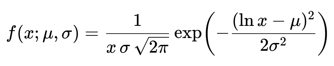
Here x is the time spent per day (strictly positive). The parameters mu and sigma represent the mean and standard deviation of the underlying normal distribution in log space. In typical scenarios, mu is influenced by the central tendency in log scale, while sigma indicates how spread out the time usage is in log scale. Although lognormal is a plausible modeling choice, real-world data might still deviate and exhibit a more general heavy-tailed nature.
In describing a skewed distribution, it is often more illuminating to look at measures like the median instead of just the mean. The mean can be misleadingly pulled up by long-tail users who spend significant amounts of time on the platform, whereas the median offers a better sense of the central user’s behavior. Another useful measure is the mode, which can reveal the most common amount of daily usage time. Dispersion metrics such as the interquartile range or standard deviation also shed light on variability. Quantiles (for example, 25th, 75th, 90th, 95th percentiles) provide additional understanding of the extremes of the distribution, particularly in a long-tail setting.
Examining changes in these metrics over time or across segments helps reveal trends or shifts. For instance, an increase in the tail’s length over a period might indicate that a new feature is prompting a subset of users to remain on the platform longer. Segment-level analysis (such as by user demographics, device type, or usage purpose) can highlight different usage patterns and inform product decisions or targeted interventions.
What If The Distribution Is Not Lognormal?
Some real-world data could exhibit a distribution that does not closely align with a lognormal curve but is still heavily skewed. In such cases, it might be more appropriate to try gamma, Weibull, or even a mixture model. Validating the fit involves techniques like quantile-quantile plots and goodness-of-fit tests to confirm how well a proposed model captures actual usage data. If user behavior changes seasonally or over time (for example, daily usage might rise during holidays), a single distribution might not suffice without dynamic modeling to adjust to these temporal patterns.
How To Choose The Right Metrics?
In a skewed setting, summarizing the distribution with multiple measures beyond just mean and standard deviation is essential. Median offers a robust central tendency measure. The interquartile range is more robust than the standard deviation to capture spread because it only focuses on the middle 50 percent of users. Higher order percentiles highlight heavy users. In some analyses, one might look at the 90th or 95th percentile usage to identify power users. Graphical methods like box plots or violin plots can visually illustrate the distribution’s skew and outliers in a way that a simple mean or standard deviation cannot.
Potential Follow-Up Questions
How can you justify that the distribution is likely to be right-skewed?
In day-to-day usage, the majority of users exhibit moderate activity, but there exists a subset who stay for considerably longer sessions, causing a large tail. This real-world observation is consistent with many human-driven processes where activities follow a heavy-tailed distribution rather than the symmetrical patterns seen in strictly controlled or naturally bounded phenomena.
When investigating whether the distribution truly skews to the right, one can empirically examine raw usage data through density plots or cumulative distribution plots. These visual checks are typically the first step toward confirming that there is a tail extending to higher usage times.
Why is the median more meaningful than the mean for this distribution?
For a heavily skewed distribution, the mean can be distorted by a small proportion of extremely high-usage individuals. The median, on the other hand, is more robust because it indicates the central point where half of the user base spends less time and the other half spends more. This is especially valuable in business or product contexts where decisions might target the average user’s experience, and the median more closely captures that “typical” user experience.
What if usage patterns differ significantly across user segments or over time?
Substantial differences in usage can arise based on demographics such as age, region, or user intent. Segment-specific distributions might each have unique shapes, potentially more or less skewed than the overall user base. It might also be that new product features, holidays, or global events shift usage patterns. One strategy is to create separate models or separate sets of descriptive statistics for each demographic or usage segment, or to use time series analysis to account for temporal changes. This approach can provide more targeted insights and improve the accuracy of business or product decisions.
How might you gather data on user time spent reliably?
A practical concern is the reliability of measuring how much time users spend on the platform. Server logs can track session lengths, but they might overestimate if users simply leave the site open. Client-side tracking using browser events or mobile app activity signals can more accurately capture active usage. Sampling bias must be considered, since not all data sources might be equally accessible or might skew toward certain device types or regions. Ensuring user privacy and data security is also paramount, and aggregated, anonymized metrics are often used in production settings.
What are potential pitfalls when summarizing usage with a single number?
Relying on a single metric, like the average, could hide critical information about distribution shape. Product teams might incorrectly optimize for one dimension of usage without realizing there is a high variation in user behaviors. Shifts in the tail (like a small group significantly increasing usage) could substantially affect the mean even if the overall user base remains stable. Reporting only the median might mask substantial increases at the high end. It is often best to report a blend of measures, including median, mean, percentiles, and even visual representations of the entire distribution.
Below are additional follow-up questions
How would you account for extreme outliers that might be artificially inflating your estimates?
An initial approach is to identify potential outliers by looking at high percentiles, for instance the 99th or 99.9th percentile, to determine whether exceptionally long usage times are legitimate. True outliers (e.g., automated bots or users who leave the site open overnight) may not reflect typical human usage. Depending on the business or product context, you can either exclude such data points or mark them for separate analysis.
A pitfall is excluding real, highly engaged power users who might matter for certain product features (like monetization or community moderation). On the other hand, including obviously spurious data (for example, multiple sessions merged into one) can distort metrics such as the mean. A carefully considered approach might be capping the maximum usage at a chosen percentile, but one must transparently document any capping or trimming process to ensure reproducibility and clarity for stakeholders.
How might changes in user base demographics or platform features shift the distribution over time?
Major shifts in demographics (for example, older adult users joining the platform or younger users leaving) or new features (like video streaming or marketplace capabilities) can cause substantial changes in daily usage time. This often shifts the distribution’s shape, potentially making it more or less skewed.
One subtlety is that the shift may not be uniform across all user segments. You could see an abrupt increase in usage for one demographic if a feature appeals specifically to them, while the rest of the distribution remains largely unchanged. Monitoring the distribution at regular intervals and segmenting by user groups, user acquisition cohorts, or features is crucial to detect and adapt to these shifts.
If we use a modeling approach (e.g., a lognormal model), how can we validate its goodness of fit thoroughly?
A rigorous validation approach starts by splitting the data into training and test sets or using cross-validation. Then, plot quantile-quantile charts comparing the observed data’s distribution to the proposed lognormal distribution. Examine whether the plotted points align closely with the reference line—if there is substantial deviation, it may indicate an ill-fitting model.
Additionally, you can use statistical tests like the Kolmogorov–Smirnov test or the Anderson–Darling test, although these can be sensitive to sample size. A large dataset may fail these goodness-of-fit tests for minor discrepancies. Visual inspection, domain knowledge, and how well the model explains user behavior trends all play important roles in deciding if the lognormal assumption is valid. A pitfall here is to over-rely on p-values without also conducting a thorough visual and domain-centric investigation.
What if a user is active on multiple devices or sessions in a single day?
Many users access Facebook from multiple devices (smartphone, desktop, tablet). If your tracking system is not consolidated across these devices, the same individual’s usage might be split across separate sessions, or mistakenly aggregated into one huge session if the tracking does not break it up properly.
To handle this, you need robust user-level identification and session merging rules. One approach is to rely on user account logins rather than device cookies, enabling you to unify usage from all devices. Another approach is to define session timeouts that split usage into distinct sessions if there has been no interaction for a certain time. A pitfall is setting a session timeout too short, artificially inflating the number of sessions, or too long, merging logically separate sessions into one. Both extremes can lead to biased estimates of daily usage patterns.
How do privacy or data retention policies affect measuring and modeling daily usage?
Strict privacy regulations may impose data minimization requirements that prevent you from retaining detailed per-user activity logs indefinitely. You might only be allowed to keep aggregated statistics or anonymized data. This can limit the granularity with which you can detect usage patterns or identify outliers. Furthermore, data retention policies can change over time, forcing rethinking of historical comparisons.
A real-world concern is that you might need to anonymize usage data so thoroughly that it hinders segmentation by user attributes such as age or location, eliminating crucial context. Balancing user privacy with detailed analysis demands careful planning, possibly including synthetic data generation for modeling purposes while preserving some features of the real distribution.
Could user behavior during weekends or holidays be drastically different, and how do you account for that?
Daily usage might be significantly higher on weekends or holidays because people have more free time. Failing to separate weekday vs. weekend or holiday usage might blend two or more distributions, where one distribution is typical weekdays and another is weekends/holidays with higher or lower usage. A single distribution can become artificially multimodal or have a more pronounced tail.
One approach is to label your data with the day of the week or holiday indicators and then build separate models or descriptive statistics for each group. This segmentation can help you understand how usage patterns differ and whether an apparent “outlier” on a weekday might be normal for a weekend. A subtlety is also seasonal behavior: some holidays or vacation periods vary by region (e.g., summer breaks) and can shift usage in ways that differ from shorter events like a single holiday.
In a real-time dashboard, how can rapid user growth or sudden viral trends distort the perceived distribution?
During sudden spikes in sign-ups—perhaps due to a marketing campaign or viral event—new users may have different usage patterns, typically shorter initial sessions as they familiarize themselves. If you’re pooling their usage data with existing users, the distribution might show a temporary dip in average or median usage. Over time, these new users might ramp up (or abandon the platform).
A pitfall is misinterpreting temporary changes in the distribution as a long-term trend. To handle this, many teams track metrics for new users separately (cohort analysis) and only merge them into overall usage statistics after a ramp-up period. This approach helps distinguish structural shifts from short-lived spikes.
If the data suggests multiple peaks in the distribution, how do you make sense of that?
A single-peaked distribution is often assumed by default (like a lognormal with one mode). However, real usage data might reveal multiple distinct peaks—for instance, a small daily usage peak around casual, infrequent check-ins, and a second peak where power users group. This phenomenon is known as a multimodal distribution and might indicate multiple subpopulations or usage contexts.
A viable approach is to investigate user segmentation to see if you can split the data into meaningful cohorts that each have a unimodal distribution. Potential cohorts might be by demographic, by user intent (entertainment vs. professional networking), or by device type. A pitfall is forcing a single distribution model to capture multiple distinct user behaviors, which can mask important product insights and hamper feature design targeted at specific subpopulations.