ML Interview Q Series: Chernoff Bound for Poisson Upper Tail Probability P(X ≥ c)

Browse all the Probability Interview Questions here.

Let X be a Poisson-distributed random variable with expected value λ. Give a Chernoff bound for P(X ≥ c) when c > λ.

Short Compact solution

To find a Chernoff bound for P(X ≥ c), we use the moment generating function M_X(t) = E[e^tX] of the Poisson distribution and the classical approach:

1. Note that M_X(t) = exp( λ(e^t - 1) ).

2. We look at min_{t > 0} e^-ct M_X(t). Define a(t) = c t + λ(1 - e^t) for t ≥ 0.

3. Because c > λ, this function a(t) starts at 0 for t = 0, initially increases, and then goes to -∞ as t → ∞. By setting its derivative to zero, we find t = ln(c/λ).

4. Substituting t = ln(c/λ) back into e^-ct M_X(t) yields the bound:

   

   Comprehensive Explanation

   The Moment Generating Function of a Poisson(λ)

   The Poisson random variable X with parameter λ has the moment generating function (MGF):

   

   for any real t. Here:

   • λ(e^t - 1) is simply λ multiplied by (e^t - 1).

   • M_X(t) is valid for all real t (though for most exponential bounds we consider t ≥ 0).

   Strategy for the Chernoff Bound

   A standard Chernoff bound for a random variable X (taking nonnegative integer values in the Poisson case) is based on:

   

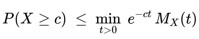
   This inequality leverages Markov’s inequality in its exponential form. The idea is to choose t > 0 that minimizes the expression e^-ct M_X(t).

   Setting Up the Optimization

   Substitute M_X(t) = exp( λ(e^t - 1) ):

   P(X ≥ c) ≤ e^-ct * exp( λ(e^t - 1) ).

   Rewrite the exponent by defining a(t) = c t + λ(1 - e^t) (note the sign carefully inside the exponent, since we are combining - c t with λ(e^t - 1)):

   Hence e^{-c t} M_X(t) = exp( -c t + λ(e^t - 1) ) = exp( λ - a(t) ).

   Thus minimizing e^-ct M_X(t) is equivalent to maximizing a(t) = c t + λ(1 - e^t) or minimizing -a(t).

   Finding the Critical Point

   We seek t > 0 that sets da/dt = 0:

   • d/dt [ c t ] = c.

   • d/dt [ λ(1 - e^t) ] = - λ e^t.

   So da/dt = c - λ e^t.

   Set that to 0:

   c - λ e^t = 0 ⇒ e^t = c / λ ⇒ t = ln(c / λ).

   Since c > λ, ln(c / λ) > 0, so indeed t = ln(c/λ) is in the domain (0, ∞) we are considering.

   Substituting Back

   At t = ln(c/λ):

   • e^t = c/λ

   • e^{-c t} = e^{-c ln(c/λ)} = (e^ln(c/λ))^-c = (c/λ)^-c = (λ/c)^c

   • M_X(t) = exp( λ( (c/λ) - 1 ) ) = exp( c - λ ).

   Hence:

   e^-ct M_X(t) = (λ/c)^c e^{c - λ}.

   Since this critical point provides the minimal value of e^-ct M_X(t) for t > 0, we conclude:

   

   This is the Chernoff bound for a Poisson(λ) random variable at threshold c > λ.

   Interpretation

   • The factor (λ/c)^c decays rapidly for c much larger than λ, capturing the small probability that a Poisson(λ) random variable substantially exceeds its mean.

   • The exponential term e^c-λ adjusts the overall scaling to account for how tails of a Poisson distribution behave.

   Example Computation in Python

   Below is a quick illustration of how one could numerically compare the Chernoff bound to the true Poisson tail probability for given λ and c.

   import math
   from math import exp
   
   def chernoff_poisson_upper_bound(lmbd, c):
       # c > lmbd
       return (lmbd / c)**c * exp(c - lmbd)
   
   def true_poisson_tail_prob(lmbd, c):
       # True probability using sum of PMF or specialized library
       from math import factorial
       # or use scipy.stats.poisson.sf(c-1, lmbd) for x>=c
       p = 0.0
       for k in range(c, 200):  # truncated for demonstration
           p += (lmbd**k * exp(-lmbd)) / math.factorial(k)
       return p
   
   lmbd = 10
   c = 20
   
   bound_val = chernoff_poisson_upper_bound(lmbd, c)
   true_val = true_poisson_tail_prob(lmbd, c)
   print(f"Chernoff Bound: {bound_val}")
   print(f"True Probability: {true_val}")
   

Additional Follow-up Question 1

What is the intuition behind exponentiating the random variable (i.e., using e^tX) in deriving Chernoff bounds?

When we use Markov’s inequality in the form:

P(X ≥ c) = P(e^tX ≥ e^tc) ≤ E[e^tX] / e^tc,

we are essentially exploiting the fact that exponentiation turns a condition “X ≥ c” into “e^tX ≥ e^tc”. Exponential growth makes large deviations in X even more significant in e^tX, so bounding E[e^tX] tightly helps to control tail probabilities. This technique (sometimes called the “exponential moment method”) is particularly strong for variables with certain moment generating functions that are known or can be easily bounded.

Additional Follow-up Question 2

Why do we specifically use the point t = ln(c/λ) for the Poisson Chernoff bound instead of any other value of t?

Because the function we are minimizing, e^-ct M_X(t), depends on t in a smooth way. By setting the derivative to zero, we discover the t that provides the best (smallest) bound. Solving da/dt = 0 yields t = ln(c/λ). If we chose any t ≠ ln(c/λ), we would get a larger value of e^-ct M_X(t), which in turn provides a looser (i.e., less tight) Chernoff bound.

Additional Follow-up Question 3

How does this Chernoff bound compare to other tail bounds such as Markov’s inequality or Chebyshev’s inequality?

• Markov’s Inequality: P(X ≥ c) ≤ E[X]/c for X ≥ 0. For Poisson(λ), that gives P(X ≥ c) ≤ λ / c. This can be quite loose for large c because it only uses the first moment.

• Chebyshev’s Inequality: Focuses on variance and means. For Poisson(λ), variance = λ. Chebyshev’s inequality states: P(|X - λ| ≥ (c - λ)) ≤ λ / (c - λ)². This again can be loose for distributions like Poisson with exponential-like tails.

• Chernoff Bound: Exploits the moment generating function. It tends to be much tighter for distributions that concentrate around their means but still have exponential tails. For c significantly larger than λ, Chernoff bounds decay faster and give a much stronger tail estimate than Markov or Chebyshev.

Additional Follow-up Question 4

Does the Chernoff bound require c to be an integer?

In principle, the derivation does not rely on whether c is an integer. The probability P(X ≥ c) is mathematically well-defined for any real c. In practice, since X is a Poisson-distributed integer, when c is not an integer, P(X ≥ c) = P(X ≥ ⌈c⌉). Regardless, the bound holds just the same because it is derived continuously in t > 0 and does not hinge on c being integral. The final expression works the same by plugging in c ≥ λ (in real terms).

Below are additional follow-up questions

Additional Follow-up Question 1

If we want to bound P(X ≥ c) for a value of c that is actually less than λ, how would we proceed, and would the same Chernoff argument still apply?

Answer Explanation Chernoff bounds, in their most common form, are frequently discussed for the case c > λ to exploit the shape of the Poisson tail above its mean. However, the Chernoff method itself comes from:

P(X ≥ c) ≤ min_{t > 0} e^-ct E[e^tX].

Nothing in the derivation formally breaks if c < λ; you could still compute the bound by finding t that minimizes e^-ct M_X(t). In that case, the derivative with respect to t may yield a negative or zero t if c < λ. Because our minimization typically restricts t > 0, the bound you get at t = 0 might actually be trivially equal to 1. This occurs because the “best” t that sets the derivative to zero might end up being negative when c < λ, and thus lies outside the domain of the standard Chernoff approach (which relies on t ≥ 0).

In practice: • For c < λ, tail probabilities P(X ≥ c) might actually be quite large, so a Chernoff bound centered on the “upper tail” style might give a less interesting inequality. • One can adapt Chernoff bounds for “lower tail” type events (for example P(X ≤ c) with c < λ) by exponentiating -tX, but for P(X ≥ c) with c < λ, it is usually more useful to rely on other concentration inequalities.

Hence if c < λ, the standard c > λ Chernoff argument is no longer the typical approach for bounding the upper tail, and you might simply revert to alternate bounds or direct Poisson tail calculations.

Additional Follow-up Question 2

How would the Chernoff bound approach change if X is the sum of multiple independent Poisson random variables with different rates λ_i?

Answer Explanation

1. Sum of Independent Poisson Random Variables If X = X₁ + X₂ + ... + X_n, where each X_i is Poisson with mean λ_i and all X_i are independent, then X is Poisson with mean λ = λ₁ + λ₂ + ... + λ_n.

2. Moment Generating Function (MGF) The MGF of a sum of independent Poissons is the product of their MGFs. Each MGF_Xi(t) = exp( λ_i(e^t - 1) ). Multiplying them yields M_X(t) = exp( (λ₁ + λ₂ + ... + λ_n)(e^t - 1) ), which is exactly Poisson(λ) with λ = Σλ_i.

3. Chernoff Bound The same Chernoff bound procedure applies with M_X(t) = exp( λ(e^t - 1) ). One would again minimize e^-ct M_X(t) over t > 0, leading to the same final form P(X ≥ c) ≤ ( (λ)/c )^c e^(c - λ ) once c > λ.

In essence, having multiple independent Poisson components sums up to another Poisson. The form of the Chernoff bound stays identical, but conceptually λ is the total sum of all rates. This result elegantly extends to more general compound Poisson processes if the individual counting processes are independent.

Additional Follow-up Question 3

In a practical scenario where λ is unknown and we have to estimate it from data, how does that affect the Chernoff bound?

Answer Explanation

1. Estimation of λ Often, we do not know the true rate λ a priori. Instead, we might collect sample data, say X₁, X₂, ..., X_N, assumed i.i.d. Poisson(λ), and form an estimator λ̂ = (1/N) ΣX_i.

2. Plug-in Approach A common approach is to replace λ in the Chernoff bound expression with its estimate λ̂. Then we would say P(X ≥ c) ≤ ( (λ̂)/c )^c e^( c - λ̂ ), but this is no longer a strictly rigorous bound unless we also account for the uncertainty in λ̂ itself.

3. Confidence Intervals To make the bound valid with high probability, we can combine the Chernoff bound with a confidence interval for λ. For instance, we can: • Construct a high-probability interval [λ_L, λ_U] for λ. • For upper tail bounding, pick the upper estimate λ_U (since c > λ is typical) and plug that into the Chernoff bound. This ensures that with high probability, we do not underestimate the true mean.

4. Conservative Bound Typically, using an upper estimate of λ or a robust approach ensures that the bounding technique remains valid. However, one must pay a price in tightness, since incorporating estimation uncertainty usually makes the bound looser.

Additional Follow-up Question 4

Can we apply the same Chernoff bound concept to distributions other than Poisson, and does the resulting formula differ?

Answer Explanation

1. General Chernoff Method The Chernoff bounding technique applies to any nonnegative random variable X whose moment generating function (or a related transform) is known or can be bounded. It does not require X to be Poisson specifically.

2. Different MGF For a general distribution, we write: P(X ≥ c) ≤ min_{t > 0} e^-ct E[e^tX]. The exact result depends on the form of E[e^tX].

3. Poisson-Specific Form For Poisson, we get the neat expression (λ/c)^c e^c-λ. If X has some other distribution (e.g., Binomial, Gamma, Sub-Gaussian, etc.), you get a different final function of t. In practice, one still picks t that minimizes e^-ctM_X(t).

4. Examples

   • Binomial Chernoff Bound: For X ~ Binomial(n, p), we use M_X(t) = (1 - p + p e^t)ⁿ.

   • Sum of i.i.d. Sub-Gaussian: We rely on bounding the MGF or cumulant generating function.

Hence, the overarching framework is the same, but the final bound formula depends entirely on the MGF or CGF specific to the distribution in question.

Additional Follow-up Question 5

Are there scenarios where the Chernoff bound might not be sufficiently tight, and can it be improved by other bounds?

Answer Explanation

1. Conservative Nature of Chernoff Bounds Chernoff bounds, while often tighter than Markov or Chebyshev, can still be conservative for certain parameter ranges. For example, if c is only slightly larger than λ (not far into the tail), or if we are looking at a distribution whose moment generating function has heavy tails or grows more quickly than the Poisson MGF, the resulting bound may not be particularly sharp.

2. Refined Large-Deviation Bounds In large-deviation theory, there are refined inequalities that sometimes yield sharper results than the basic Chernoff approach. For Poisson, one might use the so-called “exact asymptotics” or “Cramér-Chernoff” approach that yields expansions in terms of Kullback-Leibler divergences.

3. Other Tail Bounds

   • Hoeffding’s Inequality or Bernstein’s Inequality: Typically used for sums of bounded or sub-Gaussian random variables. They might yield tighter or simpler forms under certain constraints on the distribution.

   • Saddle-Point Approximations: Provide more accurate approximations to tail probabilities than Chernoff in some settings, especially when c is close to λ.

So while the Chernoff bound is a great general-purpose tool, it’s not always the absolute tightest. For extremely precise tail probability estimates, especially for moderate deviations around the mean, other specialized methods might provide sharper results.

Additional Follow-up Question 6

What are the numerical stability issues that can arise when computing the Chernoff bound for very large c, and how might they be addressed?

Answer Explanation

1. Potential Overflow and Underflow The expression (λ/c)^c e^(c-λ) can involve extremely large or extremely small numbers, depending on whether c is large, and how c compares to λ. For instance, if c is in the hundreds or thousands, (λ/c)^c might be vanishingly small, while e^{(c - λ)} might be enormous.

2. Logarithmic Computation A common technique is to take the natural logarithm of the bound: ln[(λ/c)^c e^c-λ] = c ln(λ/c) + (c - λ). This helps avoid direct exponentiation of large or tiny numbers. Once you compute the log-bound, you can exponentiate at the very end (or simply keep it in log form if that suffices for your application).

3. Software Functions

   • If using Python, the math.log function or np.log (NumPy) is typically stable for moderate c. For extremely large c, consider specialized arbitrary-precision libraries or keep the results in log form.

   • Tools like scipy.special.loggamma can help if factorials or gamma functions are involved in the derivation.

4. Practical Implications In a real-world system, you might never need to evaluate the tail probability for extremely large c far out in the tail because the event is so rare. If you do, numeric underflow might just return 0.0, which effectively conveys that the probability is exceedingly small.

Additional Follow-up Question 7

Is it possible to invert the Chernoff bound formula to solve for c in terms of a desired small probability δ, i.e., find c such that P(X ≥ c) ≤ δ?

Answer Explanation

1. Problem Formulation We want c satisfying ( (λ)/c )^c e^(c - λ ) ≤ δ. This is basically inverting the function f(c) = ( (λ)/c )^c e^(c - λ ).

2. Logarithmic Approach Taking natural logs on both sides: ln[f(c)] = c ln(λ/c) + (c - λ) ≤ ln(δ). Let g(c) = c ln(λ/c) + c - λ. Then we want g(c) ≤ ln(δ).

3. Numerical Solvers Because g(c) is not a simple linear function, we typically rely on numerical methods:

   • Newton-Raphson iteration.

   • Binary search if c is known to be in some reasonable range.

4. Interpretation

   • For large λ, the function c ln(λ/c) + c - λ can have multiple behaviors depending on c.

   • Because Chernoff bounds are not always exact, the resulting c might be a conservative estimate for the actual quantile. Still, it provides an analytical handle on “which c ensures the tail probability is at most δ?”

5. Practical Tip In real applications, you might do:

   • Start with an initial guess c₀ = λ + some multiple of sqrt(λ), or a rough percentile.

   • Iterate numerically until the difference g(c) - ln(δ) is within a small tolerance.

That inversion process can be invaluable when designing thresholds or alarms in systems needing guaranteed small false positive rates.