


ML Interview Q Series: Circle Area PDF via Variable Transformation from Uniform Radius
Browse all the Probability Interview Questions here.
19. Say you pick the radius of a circle from a uniform distribution between 0 and 1. What is the probability density of the area of the resulting circle?
Understanding the Problem and Core Concept
When the radius (r) is picked uniformly from the interval ([0,1]), the area (A) of the circle is given by the formula (A = \pi r^2). Because (r) is itself a random variable, the area becomes a derived random variable through this transformation. We want to find the probability density function (pdf) of (A).
Key Observations
The variable (r) ranges from 0 to 1. Therefore, the possible values of (A = \pi r^2) range from 0 to (\pi). Consequently, the area (A) is supported on the interval ([0, \pi]).
Transformation Approach
We use the standard method for transforming a random variable. Suppose (A = g(r)) for some function (g). If (r) has pdf (f_r(r)) and (g) is monotonic, then the pdf of (A) is:
[
\huge f_A(a) ;=; f_r\bigl(g^{-1}(a)\bigr); \left|, \frac{d}{da}\bigl(g^{-1}(a)\bigr)\right|. ]
In our problem, (g(r) = \pi r^2). Hence (A = \pi r^2). We solve for (r):
[
\huge r ;=; \sqrt{\frac{A}{\pi}}. ]
Since (r) is uniform on ([0,1]), its pdf is
[
\huge f_r(r) ;=; \begin{cases} 1 & \text{if } 0 \le r \le 1,\ 0 & \text{otherwise.} \end{cases} ]
Therefore, for a given (A) in ([0,\pi]), the corresponding (r = \sqrt{\frac{A}{\pi}}) is certainly in ([0,1]). Next, we compute the derivative:
[ \huge \frac{d}{dA}\Bigl(\sqrt{\tfrac{A}{\pi}}\Bigr) ;=; \frac{1}{2\sqrt{\pi A}}. ]
Hence the pdf of (A) for (0 \le A \le \pi) becomes:
[
\huge f_A(A) = f_r\bigl(\sqrt{\tfrac{A}{\pi}}\bigr) \times \frac{1}{2\sqrt{\pi A}}. ]
Since (f_r\bigl(\sqrt{\tfrac{A}{\pi}}\bigr) = 1) (because (\sqrt{\tfrac{A}{\pi}} \in [0,1]) for (A \in [0,\pi])), we have:
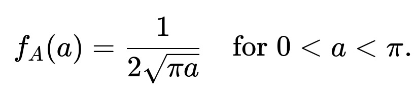
It is 0 otherwise (i.e., outside the interval ([0,\pi])).
Detailed Explanation and Sanity Checks
The pdf (f_A(a)) must integrate to 1 over its domain ([0,\pi]). We can verify that:
[ \huge \int_{0}^{\pi} \frac{1}{2\sqrt{\pi a}} , da = 1. ]
One way to see this quickly is via substitution (u = \sqrt{a}). This confirms that the function is a valid pdf.
Therefore, the probability density function for the area (A) of the circle, when its radius is chosen uniformly between 0 and 1, is:
[
\huge f_A(a) = \begin{cases} \dfrac{1}{2,\sqrt{\pi a}}, & 0 < a < \pi, \ 0, & \text{otherwise}. \end{cases} ]
That completes the direct answer to the question.
Practical Illustration in Python
Below is a small snippet to illustrate how you might empirically check or simulate this distribution:
import numpy as np
import matplotlib.pyplot as plt

# Number of samples
N = 10_000_00

# Sample radii uniformly
r_samples = np.random.uniform(0, 1, N)

# Compute areas
A_samples = np.pi * (r_samples**2)

# Plot histogram of the sampled areas
plt.hist(A_samples, bins=100, density=True, alpha=0.5, label='Sampled distribution')

# Theoretical PDF for A in [0, π]
def f_A(a):
    return 1.0 / (2.0 * np.sqrt(np.pi * a))

# Plot the theoretical pdf
a_range = np.linspace(1e-6, np.pi, 1000)
plt.plot(a_range, f_A(a_range), 'r-', label='Theoretical PDF')
plt.legend()
plt.show()
This simulation, given enough samples, should show that the histogram of sampled areas approximates the curve of (f_A(a) = \tfrac{1}{2\sqrt{\pi a}}) between 0 and (\pi).
Potential Follow-up Question 1: Could the area exceed (\pi)?
No, since the radius (r) cannot exceed 1, the maximum area is (\pi \times 1^2 = \pi). This is why the support for (A) is exactly from 0 up to (\pi).
Potential Follow-up Question 2: What if the radius was chosen from a different distribution?
Then we would apply the same general transformation technique. If (r) has a known pdf (f_r(r)) and (A = \pi r^2), we solve (r = \sqrt{A/\pi}) and compute
[
\huge f_A(a) = f_r\left(\sqrt{\tfrac{a}{\pi}}\right) \times \left|\frac{d}{da}\sqrt{\frac{a}{\pi}}\right|. ]
The specific form depends on the original distribution (f_r).
Potential Follow-up Question 3: How might one verify the distribution is properly normalized?
We check the integral:
[ \huge \int_{0}^{\pi} f_A(a), da ;=; \int_{0}^{\pi} \frac{1}{2\sqrt{\pi a}} , da. ]
Through an appropriate variable substitution ((u = \sqrt{a}), (du = \tfrac{1}{2\sqrt{a}}da)), this integral evaluates to 1, confirming it is normalized.
Potential Follow-up Question 4: How do we intuitively understand the shape of this pdf?
When (r) is uniform, smaller radii occur just as often as larger ones. But the relationship to area is quadratic. A small change in (r) when (r) is large can produce a big change in (A). In effect, more “radius space” gets mapped near the upper end of the area domain, and the pdf shape (\tfrac{1}{\sqrt{a}}) near (a=0) reflects that a lot of small radii produce small areas, compressed into a small interval near 0. This results in a higher density near (a=0), decreasing as (a) grows toward (\pi).
Potential Follow-up Question 5: How would one compute the expected value of (A)?
The expectation of (A) is
[
\huge E[A] ;=; \int_{0}^{\pi} a , f_A(a), da. ]
We can also do this directly from (A = \pi r^2) and knowledge that (E[r^2]) for a uniform ([0,1]) variable is (\tfrac{1}{3}). Hence:
[
\huge E[A] = \pi E[r^2] = \pi \times \frac{1}{3} = \frac{\pi}{3}. ]
This matches what you would get by performing the integral with (f_A(a)).
That resolves the main and follow-up questions in detail.
Below are additional follow-up questions
Potential Follow-up Question 1: How does the probability density function behave near the boundaries of the area’s support, particularly very close to 0 and very close to (\pi)?
When the radius is picked uniformly from 0 to 1, the transformed area (A = \pi r^2) takes values in ([0, \pi]). Because the pdf is derived as [ \huge f_A(a) = \frac{1}{2\sqrt{\pi a}}, \quad 0 < a < \pi, ] it has specific boundary behaviors:
Near (a = 0): The term (\frac{1}{\sqrt{a}}) goes to infinity as (a \to 0). In practical numerical computations, very small (a) values can cause large spikes in the computed probability density. This is not a sign of something invalid about the pdf (it is normal for valid pdfs to approach infinity near certain boundaries), but it can lead to numerical issues if one is trying to evaluate (f_A(a)) for extremely small (a). For instance, in floating-point arithmetic, you might run into underflow or overflow if you are not careful with how you handle (\sqrt{a}).
Near (a = \pi): As (a \to \pi), the expression (\frac{1}{\sqrt{\pi a}}) approaches (\frac{1}{\pi}). Although the function remains finite and well-defined, practically one might encounter slight floating-point inaccuracies, especially if the difference between (a) and (\pi) becomes extremely small. The function itself is well-behaved in this region, but a naive integration scheme might require higher resolution near the endpoints to ensure accuracy.
Pitfalls and Edge Cases:
If someone attempts to numerically estimate the pdf by direct evaluation for (a) near 0, they might get extremely large values (approaching infinity). The distribution remains integrable, so it is still a valid pdf.
In simulation, if you are using binning near 0, you might see very high peaks in your histogram for the area, which could be misinterpreted if not understood properly.
In real-world computations, a common practice is to add a small offset or use specialized integration/binning schemes near 0 to avoid extreme ratio blowups.
Potential Follow-up Question 2: How can we confirm empirically that the area distribution follows the theoretical pdf if we only have indirect measurements of the circle (e.g., measuring area directly instead of radius)?
Sometimes, in a real-world scenario, you might not measure the radius at all. Instead, you might measure the area of multiple circles directly (e.g., using an imaging system or some other sensor). If you are told that these circles were generated by picking a radius uniformly from 0 to 1, you need to verify that the observed areas actually follow the derived distribution (f_A(a) = \tfrac{1}{2\sqrt{\pi a}}).
Steps to confirm:
Histogram vs. Theoretical PDF: Collect the observed areas, build a histogram of the data, and compare it to the theoretical pdf over ([0,\pi]). Although the histogram may not match perfectly due to finite samples, one would expect approximate agreement in the shape of the distribution, especially with large sample sizes.
Statistical Tests: Apply goodness-of-fit tests (e.g., the Kolmogorov-Smirnov test) to see whether the sampled distribution differs significantly from the theoretical distribution.
Pitfalls:
Measurement noise could distort the observed distribution, leading to slight mismatches from the theoretical pdf. For instance, over- or under-estimates in measured area might blur the edges or add offsets.
If the data show systematic deviations, it might indicate the radius was not truly uniform or was limited in some unknown subrange.
Potential Follow-up Question 3: What happens if the radius is drawn from a uniform distribution ([0, R]) for some (R > 1)? How does that affect the derived distribution of the area?
If the radius is still uniform, but now on ([0, R]) with (R > 1), the area distribution becomes (A = \pi r^2) with (r \in [0, R]). Hence, (A \in [0, \pi R^2]). Repeating the transformation approach:
Solve (a = \pi r^2) for (r): (r = \sqrt{\frac{a}{\pi}}).
The pdf of (r), (f_r(r) = \frac{1}{R}) for (0 \le r \le R).
The pdf of (A) is: [ \huge f_A(a) ;=; f_r\Bigl(\sqrt{\tfrac{a}{\pi}}\Bigr) ; \left|\frac{d}{da}\sqrt{\frac{a}{\pi}}\right| = \frac{1}{R} \times \frac{1}{2\sqrt{\pi a}}, ] valid for (0 \le a \le \pi R^2). Outside that interval, (f_A(a)=0).
Pitfalls:
One might forget to scale by the length of the interval ([0,R]) in the original distribution, leading to an incorrect pdf.
If (R) is very large, the majority of probability mass for the area might be well beyond (\pi), changing the shape and scale significantly.
Potential Follow-up Question 4: In practical Monte Carlo simulations, how could floating-point precision errors impact the estimation of the pdf for small areas and large sample sizes?
Monte Carlo simulations typically involve:
Generating random (r) from a uniform(0,1) distribution.
Computing (A = \pi r^2).
Collecting samples and forming an empirical distribution or histogram.
Challenges:
Numerical Underflow/Overflow: For extremely small (r), (r^2) might get pushed down to floating-point underflow if using single-precision or half-precision floats. This can cause the computed area to become 0.0 in the simulation, artificially inflating the counts at 0.
Histogram Bin Allocation: If the number of bins near 0 is too coarse, one can miss the spike in the density near 0. Conversely, if you allocate too many bins, you risk extremely low sample counts in each bin, which introduces high variance in the density estimate.
Mitigations:
Use double-precision floating-point operations if possible.
Consider a variable bin width strategy for the histogram, with finer bins near 0 and coarser bins near (\pi).
Run enough samples (e.g., tens or hundreds of millions) if feasible to get a reliable estimate in the high-density region near 0.
Potential Follow-up Question 5: What if we considered the diameter (d = 2r) as the uniform variable in ([0,2])? How would that affect the distribution of the area?
If instead of picking the radius from ([0,1]), you choose the diameter from ([0,2]) uniformly, then the radius becomes (r = \frac{d}{2}) where (d) is uniform in ([0,2]). That also implies (r) is uniform in ([0,1]). Interestingly, in this specific scenario, it yields the same distribution for (r) as in the original question, so the area distribution would not change. The area (A = \pi r^2 = \pi \left(\frac{d}{2}\right)^2 = \frac{\pi d^2}{4}).
Pitfalls and Observations:
If you treat (d) as the primary variable and attempt to do the transformation from (d) directly to (A), you have (A = \frac{\pi}{4} d^2), with (d \in [0,2]). This transformation is exactly parallel to how (r) and (A) are related. The final pdf for (A) remains the same as before, because effectively the radius distribution is still uniform on [0,1].
A confusion might arise if someone thinks the distribution changes because you mention “diameter is uniform.” In this special case, “diameter uniform in ([0,2])” is equivalent to “radius uniform in ([0,1]).”
Potential Follow-up Question 6: How could measurement errors in the radius (or diameter) affect the final observed distribution of the area in real-world applications?
In practical measurement scenarios (for instance, physically measuring circles), measurement errors are often not negligible. Suppose the measured radius (\hat{r}) is the true radius (r) plus some random noise (\epsilon). Then the computed area based on (\hat{r}) would be (\pi \hat{r}^2), which does not necessarily preserve the exact theoretical distribution. Over many measurements, the observed area distribution might deviate from the ideal (f_A(a)).
Effects:
Bias: If the measurement error has a nonzero mean or is correlated with the true radius, the distribution of (\hat{r}) might systematically shift away from uniform. The resulting area distribution would differ from the ideal (\frac{1}{2 \sqrt{\pi a}}).
Variance: Even with zero-mean noise, the variance added to (\hat{r}) can cause a broadening of the distribution, especially in the tails. For example, very small or very large radii might be over- or under-sampled due to sensor limitations.
Practical Approaches:
Model the noise distribution of (\hat{r}) (e.g., Gaussian or uniform measurement error) and incorporate that into the transformation to derive a “noisy” pdf for the area.
Calibrate the measuring system to reduce bias or scale errors.
Potential Follow-up Question 7: What if the variable of interest is the circumference (C = 2\pi r)? Could we leverage a similar approach to derive the distribution of the circumference?
Yes, the same fundamental transformation technique applies. If (r) is uniform on ([0,1]), and (C = 2\pi r), then (C) ranges in ([0,2\pi]). The pdf of (C) is found by:
Solve (c = 2\pi r) for (r): (r = \frac{c}{2\pi}).
Compute the Jacobian: [ \huge \frac{dr}{dc} = \frac{1}{2\pi}. ]
Since (f_r(r) = 1) for (r\in[0,1]), we have [ \huge f_C(c) = 1 \times \left|\frac{1}{2\pi}\right| = \frac{1}{2\pi}, ] for (0 \le c \le 2\pi). Outside that range, it is 0.
Pitfalls:
It is easy to confuse the transformations for area and circumference. The area transformation is quadratic in (r) ((A=\pi r^2)), while the circumference transformation is linear in (r) ((C=2\pi r)). These lead to fundamentally different pdf shapes ((\tfrac{1}{2\sqrt{\pi a}}) vs. a constant for circumference).
If you simply assume circumference is also uniform without verifying, that changes the underlying radius distribution in a nontrivial way.
Potential Follow-up Question 8: How would you derive and interpret the cumulative distribution function (CDF) for the area, and how might that help in certain calculations?
For many practical tasks, the cumulative distribution function (CDF) can be more straightforward to work with than the pdf. The CDF for the area (A), denoted (F_A(a)), is:
[
\huge F_A(a) = P(A \le a) = P(\pi r^2 \le a). ]
Because (r^2 \le \frac{a}{\pi}) and (r) is uniform on ([0,1]):
[
\huge F_A(a) = P\bigl(r^2 \le \tfrac{a}{\pi}\bigr) = P\Bigl(r \le \sqrt{\tfrac{a}{\pi}}\Bigr). ]
Hence:
[
\huge F_A(a) = \begin{cases} 0, & a < 0, \ \Bigl(\sqrt{\frac{a}{\pi}}\Bigr), & 0 \le a \le \pi, \ 1, & a > \pi. \end{cases} ]
Pitfalls:
Sometimes one might confuse the factor. Notice that (F_A(a)) is (\sqrt{\frac{a}{\pi}}), not (\frac{a}{\pi}). This arises because (r^2 = \frac{a}{\pi}).
In practical coding tasks, you might prefer the CDF to quickly generate or test random samples using inverse transform sampling. For instance, if you have a uniform(0,1) random variable (U), you can solve for (A) via (U = F_A(A)). That means [ \huge A = \pi \left(U^2\right). ] Indeed, one can verify that plugging (A = \pi U^2) into the distribution yields the correct shape.
Potential Follow-up Question 9: In higher-dimensional analogs (e.g., picking the radius of a sphere or hypersphere), does the distribution of volume follow a similar approach?
Yes, if you generalize the problem to picking a radius for an (n)-dimensional hypersphere uniformly from some interval, the volume is still a power law in the radius. For instance, in 3D, the volume of a sphere of radius (r) is (V = \tfrac{4}{3}\pi r^3). If (r) is uniform on ([0,1]), you can similarly compute the pdf of (V). It will again be based on the transformation (V = \tfrac{4}{3}\pi r^3). The essential steps:
Express (r) in terms of (V).
Calculate the derivative (\frac{dr}{dV}).
Multiply by the pdf of (r).
Pitfalls:
The exponents and coefficients grow with the dimension. Failing to keep track of the correct factor in front (e.g., (\tfrac{4}{3}\pi) in 3D or the more complicated formula in (n)-dimensions) can lead to an incorrect pdf.
As dimensions increase, the geometry can lead to unintuitive distributions (e.g., the “volume concentration” phenomenon in high dimensions).
Potential Follow-up Question 10: How might errors arise if one incorrectly applies the formula (f_A(a) = f_r\bigl(\sqrt{a/\pi}\bigr) \bigl|\frac{d}{da}\sqrt{a/\pi}\bigr|) in scenarios where (\sqrt{a/\pi} \not\in [0,1])?
When we do the transformation, a crucial assumption is that the function (g(r) = \pi r^2) is monotonic in the relevant domain ([0,1]). Then (r = g^{-1}(a) = \sqrt{a/\pi}) must also lie within ([0,1]). But if we somehow apply that formula for (a) outside ([0,\pi]), we’d get (\sqrt{a/\pi} > 1) (for (a>\pi)) or an imaginary value for negative (a). The correct pdf must be set to 0 outside the valid range of (a).
Pitfalls:
Accidentally forgetting to “clip” the domain of (A) to ([0,\pi]) could produce a pdf that integrates to more (or less) than 1, invalidating the distribution.
In a coding context, if you do not handle the domain check, you might end up taking the square root of a negative number for (a < 0) or get real values for (a > \pi) that do not correspond to a valid radius in ([0,1]).
These edge conditions underscore how important it is to keep track of the domain of each random variable when performing transformations.