ML Interview Q Series: CNN Architecture Breakdown: Convolution, Pooling, and Fully Connected Layers in Image Processing.

📚 Browse the full ML Interview series here.

6. CNN Components: In a Convolutional Neural Network (CNN), what is the role of convolutional layers, pooling layers, and fully connected layers? Explain how convolutional layers detect local patterns/features using kernels, how pooling layers reduce spatial dimensions and provide translational invariance (e.g. max pooling), and how fully connected layers at the end can combine extracted features for final predictions. Also, why are CNNs well-suited for image data compared to fully connected networks?

Role of Convolutional Layers

Convolutional layers are responsible for detecting local patterns in the input. In image processing, the input is typically a grid of pixel intensities, possibly with multiple channels. A convolutional layer applies small filters (also called kernels) that slide across the spatial dimensions of the input. At each spatial location, these filters perform element-wise multiplications between their weights and the local patch of the input, summing up these products to produce an activation. Convolution exploits the idea that relevant features (such as edges, corners, textures) often repeat at different spatial locations, so learning a filter that is useful for detecting a certain pattern in one part of the image can be applied anywhere in the image.

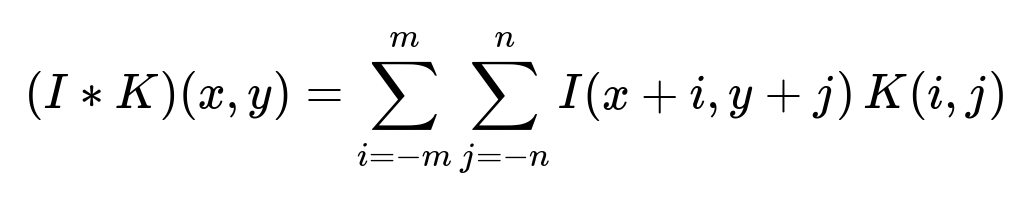
The essential mathematical description of a 2D convolution between an input image and a kernel can be expressed with summations over the spatial region. Though it can be formulated in many ways, a typical discrete 2D convolution for a pixel location (x, y) can be represented as:

In practice, frameworks often implement cross-correlation rather than a strict mathematical convolution, but the term "convolution" is used in deep learning by convention. The trainable weights in each filter adjust to detect patterns that best help minimize the overall loss function (for instance, a classification error). Deeper convolutional layers tend to learn more complex features from combinations of simpler ones. Early layers might detect edges or corners, while deeper layers might detect entire objects or complex textures.

Convolutions reduce the number of parameters compared to fully connected layers when dealing with image data, because the kernel size is typically much smaller than the image dimensions. This weight sharing (the same filter slides across the entire image) makes convolutional layers far more efficient and also improves generalization, as they exploit the spatial stationarity of local features.

Role of Pooling Layers

Pooling layers, such as max pooling or average pooling, reduce the spatial dimensions of the feature maps. Pooling is usually applied after a convolutional layer. It’s a downsampling operation in which a small window slides across the feature map and aggregates the feature responses in that window (by taking the maximum or average, for example). This yields two major benefits:

It decreases computational cost and reduces the number of parameters, because the spatial resolution becomes smaller after pooling. This smaller resolution means that subsequent layers handle fewer activations.

It brings a degree of translational invariance, because small shifts or distortions in the input will yield similar pooled feature values. Max pooling in particular can capture whether a certain feature is present within a local region, regardless of its precise location.

Pooling layers thus help the network progressively compress the spatial representation, focusing on the most relevant features and discarding minor positional details that do not significantly affect the classification outcome.

Role of Fully Connected Layers

Fully connected layers appear toward the end of many CNN architectures, although some more modern designs reduce their usage or even replace them with global average pooling. In a classical CNN pipeline, the final feature maps from the last convolution/pooling layer are “flattened” into a 1D vector. That vector is then fed into one or more dense (fully connected) layers that perform the final classification or regression. Each unit in a fully connected layer receives inputs from all the outputs of the previous layer, enabling the network to combine the spatially extracted features into high-level reasoning.

For example, if the task is to recognize objects in an image, all the localized features extracted by the previous convolutional layers are aggregated and integrated by these dense layers to produce a final prediction across classes. The final fully connected layer typically has an output dimension corresponding to the number of target classes (followed by a softmax in classification tasks).

Why CNNs Are Well-Suited for Image Data Compared to Fully Connected Networks

CNNs are very well-suited for image-related tasks due to three main reasons:

They dramatically reduce the number of parameters by exploiting local connectivity and weight sharing. Rather than connecting every input pixel to every neuron in the next layer, convolutional kernels connect only local patches, and the same kernel is applied everywhere. This prevents an explosion in the number of parameters and helps the network generalize.

They explicitly capture spatial structure. Images have strong local correlations (neighboring pixels are more closely related than distant ones). Convolution kernels take advantage of these correlations to learn local features that remain meaningful across the entire image.

They offer a built-in translational invariance (especially when combined with pooling), meaning that shifting objects in an image slightly does not drastically change the network’s internal representation. This property is very important for tasks like object recognition.

In contrast, a large fully connected network that directly takes every pixel as an input neuron would have enormous parameter counts and would not inherently exploit the spatial arrangement of pixels. Such networks often overfit and are less efficient, making CNNs the preferred choice for most image-based machine learning tasks.

How does one initialize the weights of convolutional layers effectively?

Modern deep learning practice often uses weight initialization schemes that maintain stable gradients. For convolutional layers, one commonly used approach is He initialization or Xavier (Glorot) initialization, which are designed to keep the variance of the signals and gradients roughly consistent across layers. He initialization is often used with ReLU activation functions, while Xavier initialization can be used with sigmoid or tanh activations.

He initialization sets the variance of each filter’s weights based on the number of incoming activations (fan_in). For instance, it might sample weights from a normal distribution with a variance of 2/fan_in. This approach helps address the vanishing or exploding gradient problem, because it avoids shrinking or magnifying signals excessively as they propagate forward or backward.

Another important consideration is bias initialization. By default, biases are often just initialized to zeros if there is batch normalization or a similar mechanism in the network. If not using batch normalization, sometimes a small constant might be used.

How can we visualize what features the convolutional layers learn?

Visualizing learned filters and feature maps can provide insights into what a CNN deems important. One approach is to directly inspect the learned weights of the filters in the first convolutional layer. These can often be displayed as small, interpretable patches, especially if the network is trained on natural images. Early filters might look like oriented edge detectors or Gabor-like filters capturing various spatial frequencies.

For deeper layers, one can visualize the intermediate feature maps by forwarding an input image through the network and examining the activations right after a convolution. These deep-layer feature maps can be less interpretable directly, though they often highlight complex parts of objects or textures. Another advanced technique is guided backpropagation or Grad-CAM, which focuses on important regions in the input that contribute to a particular output class. These techniques are often used in debugging or explaining CNN decisions.

Could you discuss potential pitfalls when training CNNs for image classification?

One pitfall is overfitting, particularly if the model is very deep and the training dataset is not large. Regularization techniques such as dropout, weight decay, data augmentation, and batch normalization are often essential. Another challenge is exploding or vanishing gradients, where signals become too large or too small as they pass through many layers. Approaches like careful initialization and normalizing the inputs (via batch normalization) help mitigate this issue.

Another subtle pitfall involves improper handling of hyperparameters, such as choosing a kernel size that is too large or too small for a given image resolution. Learning rate scheduling can also be important; choosing an overly large or overly small learning rate can cause slow convergence or divergence. Data augmentation strategies can also be mishandled, causing additional noise or transformations that do not reflect real data variations.

Implementation details around padding and stride can lead to unexpected dimension mismatches. For example, if you leave out padding while convolving multiple layers in a deep network, the spatial dimensions might shrink too fast. Conversely, using too much padding can yield unnecessary edge effects. Monitoring shapes and debugging dimension issues is important when building practical CNN architectures.

Could you provide a simple code example of a CNN for image classification in PyTorch?

Below is a concise example. It uses a single convolutional layer, a pooling layer, and a couple of fully connected layers. This is just a minimal illustration; in practice, deeper or more sophisticated architectures are often used:

import torch
import torch.nn as nn
import torch.nn.functional as F

class SimpleCNN(nn.Module):
    def __init__(self, num_classes=10):
        super(SimpleCNN, self).__init__()
        self.conv1 = nn.Conv2d(in_channels=3, out_channels=16, kernel_size=3, padding=1)
        self.pool = nn.MaxPool2d(kernel_size=2, stride=2)
        self.fc1 = nn.Linear(16 * 16 * 16, 128)  # For an input image of size 3x32x32
        self.fc2 = nn.Linear(128, num_classes)

    def forward(self, x):
        x = F.relu(self.conv1(x))
        x = self.pool(x)
        x = x.view(x.size(0), -1)  # Flatten
        x = F.relu(self.fc1(x))
        x = self.fc2(x)
        return x

# Example usage:
# model = SimpleCNN(num_classes=10)
# output = model(torch.randn(8, 3, 32, 32))  # batch of 8 images (3 channels, 32x32)
# print(output.shape)  # torch.Size([8, 10])

This code illustrates the essential ideas of a CNN: a convolutional layer to extract features, a pooling layer to downsample, and fully connected layers to combine features for classification. The forward pass includes activation functions (ReLU here) to introduce nonlinearity.

How do modern CNN architectures differ from the simple approach?

Modern CNN architectures (e.g., ResNet, Inception, MobileNet, EfficientNet) often include sophisticated components:

Residual connections. Networks like ResNet introduce skip connections (shortcut paths that bypass certain layers) to mitigate vanishing gradients and enable training extremely deep networks.

Inception modules. Inception designs fuse multiple convolution filter sizes in parallel, concatenating their outputs to capture multi-scale features.

Depthwise-separable convolutions. Lightweight architectures like MobileNet factorize a regular convolution into two simpler ones (a depthwise convolution and a pointwise convolution), drastically reducing computational cost while preserving accuracy.

Batch normalization. Many modern architectures apply batch normalization after convolutions to stabilize training and improve generalization.

Global average pooling. Instead of using large fully connected layers, some networks replace them with a global pooling layer (e.g., average pooling) that summarizes the spatial dimensions. This helps reduce parameter count and can improve robustness.

The fundamental ideas—local connectivity, weight sharing, and pooling—remain central, but these architectures refine and extend them to achieve better accuracy, faster training, and reduced computational complexity.

How do you handle the issue of varying input image sizes?

CNNs typically expect fixed-sized inputs, especially if the architecture ends with fully connected layers. Common solutions include resizing or cropping images to a standard dimension. Another approach is to design fully convolutional architectures that allow variable input sizes, often used in semantic segmentation tasks. In classification tasks, a common practice is to apply random crops and random resizing to augment the data during training, but at test time, one typically resizes images to a consistent shape to match the model’s input constraints.

In many real-world applications, a combination of resizing and data augmentation is used to make the model robust to scale variations. If the tasks require higher precision (e.g., medical images with critical local details), carefully chosen resizing strategies or model changes might be required. Using adaptive pooling can also help handle variable input sizes before passing features to fully connected layers.

How can we further enhance translational invariance beyond pooling?

While pooling provides a local form of translational invariance, more advanced methods include:

Strided convolutions. Instead of separate pooling layers, one can set a convolution stride greater than 1 to downsample directly while learning the downsampling kernels.

Data augmentation with translations. Randomly shifting the input images during training can improve robustness to translations. The model becomes less sensitive to small shifts because it sees multiple shifted versions of the same data.

Use of architectures like Spatial Transformer Networks. A Spatial Transformer module can learn how to warp or align features spatially. This goes beyond simple pooling to handle more general geometric transformations.

In many tasks, the combined effect of convolution, pooling/stride, and data augmentation already provides ample invariance.

How do you decide on kernel sizes, strides, and other hyperparameters for CNNs?

There is no universal formula; it usually depends on domain knowledge, experimentation, and best practices from successful architectures. Common defaults include kernel sizes of 3×3, especially in deeper architectures. Wider kernels like 5×5 or 7×7 might be used in early layers or if the input resolution is high. Smaller kernels generally reduce computational cost and preserve detail, while larger kernels can capture broader context. Stride is frequently 1 in many standard layers, with occasional strides of 2 for downsampling. Pooling layers often use a 2×2 window with stride 2. The number of filters (channels) in each layer often doubles as one moves deeper in the network to capture increasingly complex features.

Architectures such as VGG, ResNet, and others offer good reference points. VGG uses stacks of 3×3 convolutions, doubling filters at various stages. ResNet similarly uses mostly 3×3 convolutions but includes skip connections. Empirically validated designs often serve as a baseline that researchers or practitioners adapt to specific tasks.

---

Below are additional follow-up questions

How do CNNs handle color channels differently from grayscale data or multi-spectral data?

CNNs handle multiple channels by having each convolutional filter span across all input channels when performing a single 2D convolution. For example, a filter of size 3×3 operating on an RGB image is actually 3×3×3 in shape (height × width × channels). Each channel in the filter corresponds to the corresponding channel in the input (R, G, B). The result of applying this 3D kernel to the spatial region (3×3 patch in each of the R, G, B planes) produces a single scalar output, which is then combined across the spatial dimension as the filter slides over the image. This means:

• For grayscale images with 1 channel, each filter might be 3×3×1.

• For multi-spectral data (e.g., satellite imagery with multiple spectral bands), each filter includes as many channels as the input. Thus, if you have 12 spectral bands, and use a 5×5 filter, it becomes 5×5×12.

A potential pitfall arises when the dimensionality of channels is very large. If the input has many channels, each filter must still convolve across all of them, potentially increasing the parameter count significantly. One edge case is in medical imaging where a modality might have dozens or hundreds of channels (e.g., temporal frames in fMRI). Balancing the number of filters and the filter size is crucial in these scenarios to prevent ballooning memory usage and overfitting.

What if we have extremely unbalanced classes in our image classification task?

Class imbalance can severely affect model training because the CNN might become biased towards the majority class. When classes are extremely unbalanced, the network may simply learn to predict the most common label for all inputs, which might yield deceptively high accuracy but poor recall on minority classes. Strategies to address this include:

• Oversampling the minority classes. Techniques like random oversampling or generating synthetic samples (e.g., SMOTE, though SMOTE is typically used for tabular data; for images, you can use data augmentation).

• Undersampling the majority classes. This can lose valuable data but might be acceptable if the majority class is overwhelmingly large.

• Using class-weighting in the loss function (e.g., weighting the minority classes more, so that misclassifications of minority samples have a bigger penalty). For instance, many deep learning frameworks allow specifying a weight vector for each class in cross-entropy loss.

• Employing advanced augmentation. For instance, applying transformations more aggressively to minority-class images to artificially expand their dataset.

A common pitfall is forgetting to evaluate on appropriate metrics like precision, recall, F1-score, or balanced accuracy. Simply looking at the overall accuracy can mislead you. Another edge case involves extremely rare classes where you might have very few samples of a certain category, and you risk overfitting if you only use naive oversampling.

If the dataset is small, how can we prevent overfitting in CNNs and ensure generalization?

When the training set is limited, CNNs can easily memorize the dataset and fail to generalize. Key techniques to mitigate overfitting include:

• Data augmentation. This is crucial for image tasks. Randomly flipping, rotating, scaling, or color-jittering images can effectively enlarge the training data. The network learns that real images might have small variations but still represent the same class.

• Transfer learning. Using a pre-trained model (trained on a large dataset such as ImageNet) as a starting point, and then fine-tuning on the smaller dataset, often improves performance and reduces overfitting. The lower convolutional layers learn general features like edges and corners that transfer well to other tasks.

• Regularization. Techniques such as dropout, weight decay ( regularization), or adding mild label smoothing can keep the model from over-relying on specific training examples. Batch normalization also has a slight regularizing effect.

• Architectural adjustments. Instead of using a very deep network, opt for a simpler architecture if the dataset is truly small. Overly large models can memorize the entire training set.

A subtle pitfall is to rely too heavily on data augmentation without ensuring that augmented images still look realistic. Overly aggressive transformations might produce unnatural images that degrade learning. Another edge case is that in some domains (like medical imaging), the location or orientation of certain features can be critical, so random rotations or flips could remove important context.

How do you manage training CNNs on large, high-resolution images?

For high-resolution images, using a naive approach to feed them directly into the CNN might lead to extremely large memory usage and slow training. Common solutions include:

• Downsampling or cropping the images to smaller patches. This reduces memory requirements but might risk losing important global context. Strategies like random cropping can help the model see various local regions of the image.

• Using sliding-window techniques or region-based approaches if you need to detect local objects or features in the image.

• Employing patch-based training. For instance, in medical image segmentation tasks, you often extract smaller 2D or 3D patches due to memory constraints.

• Using specialized architectures or GPU memory tricks (such as gradient checkpointing) to train on large images without storing all intermediate activations.

A pitfall here is discarding too much information by downsampling. If you reduce a 4K-resolution image to a fraction of its size, you might lose critical details. Another subtlety is dealing with variable shapes. Large images might come in slightly different resolutions, forcing consistent resizing or cropping strategies.

What is the role of dilation in convolution layers, and when might it be used?

Dilation (also called atrous convolution) allows the convolutional kernel to skip certain points in the receptive field, effectively enlarging the receptive field without increasing the number of parameters. With a dilation rate dd, each kernel tap is spaced by d−1 pixels. This can be very helpful in tasks like semantic segmentation, where it’s valuable to capture context without reducing resolution too quickly.

Dilation can be mathematically expressed as:

Potential pitfalls include choosing a dilation rate that is too large, causing the filter to skip too many intermediate pixels and lose local details. Another subtlety is combining dilation with pooling or strided convolutions incorrectly, which might produce complicated or overlapping receptive fields that are hard to interpret.

How can we leverage transfer learning effectively in CNN-based solutions?

Transfer learning typically means taking a CNN pre-trained on a large benchmark dataset (like ImageNet) and reusing some or all of its weights. There are a few common strategies:

• Feature extraction: Freeze most of the convolutional layers (which capture generic low-level and mid-level features) and only train the final layers on your new dataset.

• Fine-tuning: Unfreeze some of the deeper convolutional blocks so that they can adapt to the specifics of your new data. This is especially useful when your target dataset is somewhat similar to the original dataset on which the CNN was trained.

• Layer removal or addition: Some tasks benefit from removing or modifying certain blocks, or adding new blocks like attention modules.

One pitfall is that if your domain is drastically different from the ImageNet domain (e.g., medical X-ray images vs. natural photographs), the pretrained features might be less relevant. Another subtlety is deciding how many layers to unfreeze. Fine-tuning too many layers can cause overfitting if the new dataset is small; fine-tuning too few layers may limit the network’s ability to adapt to domain-specific nuances. Finally, be sure to adjust the learning rate—often a smaller learning rate for pretrained layers is beneficial, while newly added layers can use a slightly higher rate.

Could you explain the difference between ‘same’ padding and ‘valid’ padding modes, and when each is typically used?

Use cases:

• Same padding is common when the design calls for maintaining the same resolution at each layer. This is often found in modern architectures where the network needs deeper or iterative extraction of features without losing spatial dimension quickly.

• Valid padding is simpler mathematically but reduces feature map size after each convolution. This can be helpful if you want a deliberate reduction in size or if you don’t want added border effects from padding.

A pitfall can occur if your architecture requires a certain output dimension but you use "valid" padding inadvertently. You might end up with dimension mismatches in deeper layers. Another subtlety is the impact of zero-padding at the edges, which can introduce edge effects or artificial borders that might slightly affect learned filters.

What are the differences between 1D, 2D, and 3D convolutions, and are they used in different contexts?

• 1D convolutions typically operate along a single dimension (with channels) and are common in temporal or sequence-based data (e.g., audio signals, text sequences after embedding). A 1D kernel has a shape like kernel_size × in_channels, sliding over one dimension.

• 2D convolutions are the default in most image-based CNNs. The kernel slides over both width and height dimensions (and has channels). This is ideal for typical 2D images.

• 3D convolutions extend this to an additional dimension, often time or depth. This is frequently used for video data (height, width, and time). For example, a 3D kernel might be 3×3×3 in space-time, capturing motion and spatial correlations simultaneously.

Using the wrong dimensionality leads to mismatches in how data is shaped. A common edge case is if you attempt to feed video data into a purely 2D CNN without carefully handling the time dimension, or you attempt a 3D convolution but your data has fewer dimensions than expected. Another subtlety is that 3D convolutions can be very memory-intensive, so approaches like 2D + temporal pooling or using (2+1)D convolutions (factorizing 3D convolution into separate spatial and temporal parts) might be more efficient.