
ML Interview Q Series: CNN Output Size Formula: Understanding Kernel, Stride, and Padding Effects.

📚 Browse the full ML Interview series here.
7. Convolution Output Calculation: In a CNN, how do you calculate the output size of a convolutional layer? *For example, if an input feature map is 32×32 and you apply a convolution with a 5×5 kernel, stride 1, and padding 2, what will be the dimensions of the output feature map? Show how the formula applies (output = $(\text{input\_size} + 2*\text{padding} - \text{kernel\_size})/\text{stride} + 1$).*
Overview of Convolution Output Size
When we deal with Convolutional Neural Networks (CNNs), a critical question is determining the size of the output feature map produced by each convolutional layer. This is vital for constructing architectures and ensuring dimensional consistency across layers. In particular, we often want to know how padding, stride, and kernel size affect the output spatial dimensions.
In two-dimensional convolutions (like images), each convolutional layer has three key hyperparameters that affect output height and width:
Kernel size: The spatial size of the filters (e.g., 3×3, 5×5).
Stride: The step the convolution filter moves each time (e.g., 1, 2).
Padding: The amount of zeros (or other values) padded around the input (e.g., same padding in TensorFlow terms or 'pad=1', 'pad=2' in PyTorch).
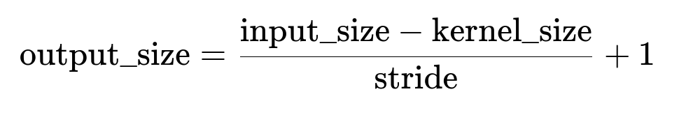
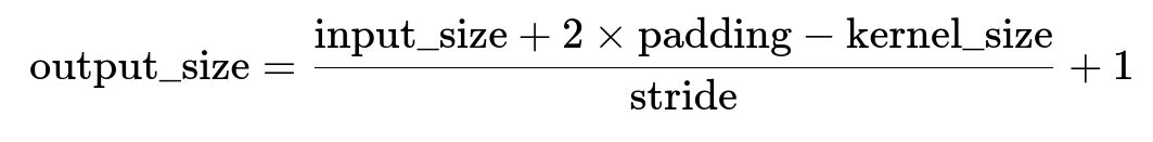
The formula to compute the output spatial dimension (width or height) in a standard (no-dilation) convolution is often stated as:

We can apply this formula independently to both the height and width dimensions if they share the same parameters, or separately if they differ.
Applying the Formula to the Example
Specific Example Parameters
Input size (width or height): 32
Kernel size: 5
Stride: 1
Padding: 2
Substituting Values
We plug in these numbers into the formula:
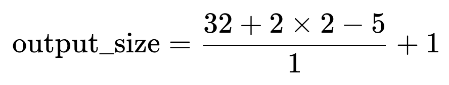
Let’s break that down:
2×padding=2×2=4
input_size+2×padding=32+4=36
Subtract the kernel size: 36−5=31
Divide by the stride (which is 1): 31/1=31
Add 1: 31+1=32
Hence, the output spatial dimension is 32.
Intuitive Explanation
Padding of 2 on each side (top, bottom, left, right) with a 5×5 kernel and stride 1 is the classic setting to preserve the spatial dimension. Essentially, by adding the right amount of padding, you let the kernel “reach” slightly beyond the borders of the original image. For a 5×5 kernel, a padding of 2 on each side in 2D preserves the original 32×32 input, yielding an output dimension of 32×32 in the spatial domain.
Detailed Reasoning About Each Parameter
Kernel Size
A 5×5 kernel means each filter will span a 5×5 region of the input. If you think of it from the center of the kernel, 2 pixels in each direction from the center covers a 5×5 patch. This is why padding of 2 is often paired with a 5×5 kernel when the stride is 1 and we want to keep the output size the same as the input size.
Stride
Stride 1 indicates that the convolutional window moves 1 pixel at a time across the input feature map. If the stride were larger (e.g., 2), the output dimension would be reduced because we skip more pixels each time we shift the kernel window.
Padding
Padding 2 means we add 2 rows of zeros (or mirrored/reflective values in more advanced schemes, but typically zeros in many frameworks) on the top and bottom, and 2 columns of zeros on the left and right. This expands the input from 32×32 to effectively 36×36, giving the 5×5 kernel enough room to “slide” in such a way that the corners of the original 32×32 are covered fully.
General Layout of Convolution Shapes
Number of Output Channels

That means if you had 64 filters, and the output spatial dimension is 32×32, the final shape is (batch_size,64,32,32)
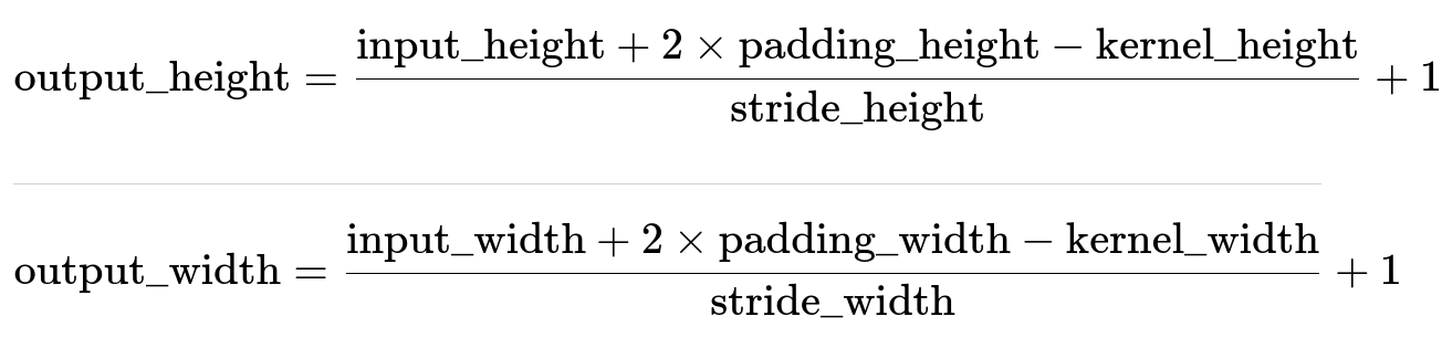
Multiple Dimensions: Height vs. Width
The same formula applies to both the height and width, though you might have separate parameters for each dimension in certain frameworks:
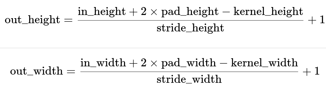
For the example in question, both the height and width used the same parameters, hence 32×32 results again.
Example in PyTorch
Below is a simple PyTorch code snippet to illustrate creating a convolutional layer with these parameters and verifying the output shape.
import torch
import torch.nn as nn

# Example input: batch_size=1, channels=3, height=32, width=32
x = torch.randn(1, 3, 32, 32)

# Convolution with kernel_size=5, stride=1, padding=2
conv_layer = nn.Conv2d(in_channels=3, out_channels=16, kernel_size=5, stride=1, padding=2)

# Forward pass
output = conv_layer(x)
print(output.shape)
# Expected: [1, 16, 32, 32] in the shape (batch_size, out_channels, out_height, out_width)
When you run this, you’ll get a shape of [1, 16, 32, 32], verifying that the spatial dimension is 32×32 while the output channels are determined by the out_channels parameter set to 16 in this example.
Common Pitfalls and Edge Cases
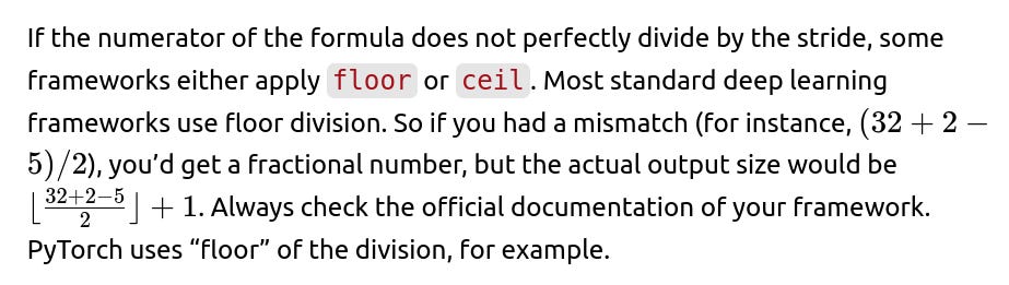
Fractional Output
Kernel Larger Than Input
If your kernel size is larger than your effective input size (e.g., a 7×7 kernel on a 5×5 input with insufficient padding), you might end up with an output dimension that is zero or even negative if you rely purely on the formula. This would typically throw an error in frameworks.
Dilation
Dilation is another parameter that can effectively enlarge the receptive field of the kernel. The formula for the output dimension in that scenario modifies the kernel size to (kernel_size−1)×dilation+1. So you would see:
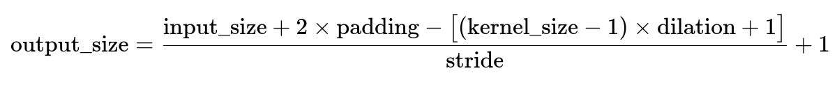
This is very common when dealing with dilated convolutions for tasks such as semantic segmentation.
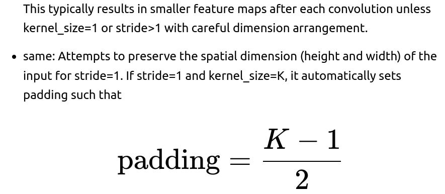
“Same” vs. “Valid” Convolutions in Other Frameworks
In TensorFlow’s “same” padding, the dimension is preserved (assuming stride 1), which basically sets the padding automatically so that the output size stays the same as input size. “Valid” padding in TensorFlow implies no padding, so the dimension shrinks if the kernel size is greater than 1.
Putting It All Together
In summary, the formula you provided:

is the fundamental reference point. For the specific example of a 32×32 input, a 5×5 kernel, stride of 1, and padding of 2, the output dimension is 32×32. This is exactly what we expect when using “same” padding logic for a 5×5 kernel with stride 1.
Follow-up Questions and Detailed Answers
What if the stride were 2 instead of 1?
If we change the stride to 2, the output size changes because we move the kernel by 2 pixels at a time:
Using the same parameters except stride=2:
Input size: 32
Kernel size: 5
Padding: 2
Stride: 2
Now we use:

2×2=4
32+4−5=31
31/2=15.5
Frameworks typically do floor division internally, so it would be 15, then add 1 for a total of 16. So:
Answer: The output dimension becomes 16×16 in that scenario.
This is a common configuration if you want to downsample the feature map. For example, in typical CNN architectures (like VGG or ResNet at certain stages), you might want to reduce the resolution by using stride=2.
How is the channel dimension affected?
The spatial dimension formula does not directly control the number of output channels. Instead, the number of filters in your convolution layer sets the output channel dimension. If your convolution has out_channels = 64, then your output shape would be:
(batch_size,64,output_height,output_width)
Internally, each filter is 5×5×(input_channels). The number of filters themselves is how you choose the final channel count.
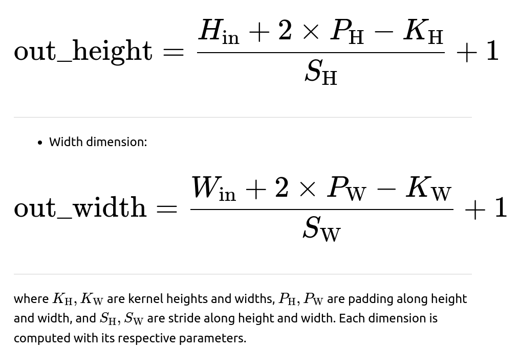
What if we have non-square inputs or kernels?
If the input is not square (e.g., 64×32 height×width) or the kernel is not square (e.g., 5×3), we apply the formula to each dimension independently. For height H and width W:
Height dimension:
How does zero-padding work under the hood?
Zero-padding simply means that before performing the convolution operation, additional rows and columns of zeros are concatenated to the edges of the input feature map. For a 2D input:
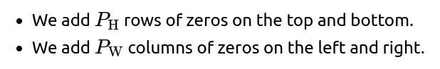
The main purpose is to control the effective size of the input so that the kernel can apply properly near the edges. Without padding, the corners or edges of the input are seen fewer times by the kernel because there is no extra “border” region.
What happens if the formula yields a negative or zero?
A negative or zero means your effective receptive field (after accounting for padding) cannot be placed even once in a valid position. In practice, frameworks like PyTorch usually throw an error such as “Calculated padded input size is not compatible with kernel size.” If it’s exactly zero, that might be a corner case: you could see a 0 dimension in some frameworks. Usually you want to design your network so that doesn’t happen.
Could the formula produce a fractional result?
Yes, if (input_size+2×padding−kernel_size) is not divisible by stride, you get a fractional result. As mentioned, the official formula in many deep learning frameworks performs floor on that fraction. In math notation, it is effectively:

This ensures you always get an integer. That’s why careful design is needed if you want to exactly match certain output dimensions. For instance, you might adjust padding or stride to ensure it divides properly.
How does dilation factor into the formula?
If we incorporate dilation d, the kernel “expands” so that its effective size is (kernel_size−1)×d+1. This is often used in tasks that require large receptive fields (like semantic segmentation with Dilated (Atrous) Convolutions). The revised formula:

That means with dilation, each “gap” within the kernel is expanded by d−1, increasing the receptive field without adding to the number of parameters significantly.
How do we implement these calculations in an actual CNN architecture design workflow?
In practice, you usually:
Choose your kernel size, stride, and padding to achieve the desired receptive field and dimension transformations.
Use the formula to verify that the output dimension is correct.
Construct your code in a framework (PyTorch, TensorFlow, etc.).
Print or log the layer outputs to confirm you’re getting the dimensions you expect.
Modern deep learning frameworks handle much of this automatically once you specify the hyperparameters. However, thoroughly understanding this formula is important to debug issues, create custom architectures, or interpret advanced designs like dilated or transposed convolutions.
Summary
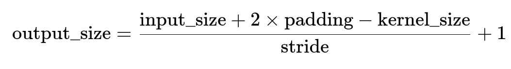
The canonical formula for computing the output dimension of a convolutional layer is:
In practice, a floor operation is used internally for non-integer results.
In the given example, with a 32×32 input and a 5×5 kernel, stride=1, padding=2, the output spatial dimension remains 32×32.
This is the typical scenario for “same” style convolutions where you keep the output dimension the same as the input dimension if you choose padding appropriately.
Remember that the number of output channels is controlled by the number of filters in the convolution, not by the spatial dimension calculation.
When designing CNNs, always confirm that stride, padding, and kernel size yield the desired dimensions. Be aware of edge cases involving fractional results, negative output sizes, or large dilations.
Additional Follow-up Question
How do we verify the convolution output dimensions in a more real-world scenario involving multi-layer networks?
In real-world CNN architectures, you typically have many consecutive layers. You can:
Construct a dummy input tensor of shape (batch_size,in_channels,H,W).
Sequentially pass it through each layer (convolution, pooling, activation, etc.) in a forward pass.
Print out the shapes after each layer to confirm they match your expectations.
For instance, in PyTorch:
import torch
import torch.nn as nn

class SimpleCNN(nn.Module):
    def __init__(self):
        super(SimpleCNN, self).__init__()
        self.conv1 = nn.Conv2d(in_channels=3, out_channels=16, kernel_size=5, stride=1, padding=2)
        self.conv2 = nn.Conv2d(in_channels=16, out_channels=32, kernel_size=3, stride=2, padding=1)
        # Additional layers...

    def forward(self, x):
        x = self.conv1(x)
        print("Shape after conv1:", x.shape)
        x = self.conv2(x)
        print("Shape after conv2:", x.shape)
        # ...
        return x

model = SimpleCNN()
dummy_input = torch.randn(1, 3, 32, 32)
output = model(dummy_input)
By running such code, you see the transformations step by step. This is exactly how you ensure that the formula you use on paper matches the actual computations performed by the framework.
That covers the essence of how we calculate the output size of a convolutional layer and how the provided formula applies to the question’s specific example of a 32×32 input, 5×5 kernel, stride 1, and padding 2.
Below are additional follow-up questions
How does grouping (grouped convolutions) affect the output size calculation?
When using grouped convolutions in frameworks like PyTorch (by setting the "groups" parameter greater than 1 in a 2D convolution), the convolution operation is divided into separate groups of channels. Despite this internal grouping, the spatial dimensionality calculation for the output remains governed by the same formula:
So the grouped convolution only changes how many channels each group processes, not the height/width output shape. However, a potential pitfall is ensuring the “in_channels” parameter is divisible by the number of groups. For instance, if you have in_channels=32 and groups=8, you must have 32 % 8 == 0. The same condition applies for out_channels if the framework requires it (e.g., in_depth and out_depth each divisible by groups in a depthwise scenario). If you don’t satisfy those channel divisibility constraints, you’ll face dimension mismatch errors or framework exceptions.
How do “valid” and “same” padding differ in frameworks beyond PyTorch?
In frameworks like TensorFlow/Keras:
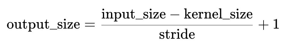
valid: Means no padding around the input, so each convolution reduces the spatial size if kernel_size > 1. Using the formula:
for odd K. For even K, the padding is computed in a way that the output dimension remains close to the input dimension, often using floor or ceiling to handle fractional offsets.
A subtle real-world issue is that “same” padding can produce off-by-one dimension changes if stride > 1 and kernel_size is even. You may see that your final dimension is 1 pixel off from what you might have anticipated, depending on how the framework splits the padding above/below or left/right. Always verify the final shape with actual code or check the official documentation to see whether the library floors or ceilings during the padding split.
How does a non-square kernel, like 3×7, change the calculation?
If your kernel is 3×7, you apply the standard formula independently for height and width. For example, if the input is 64×32 (height×width) and you have kernel_height=3, kernel_width=7, stride=1, padding_height=1, padding_width=3, then:

Hence you can preserve the dimensions in the height while using a bigger kernel in the width. One subtle pitfall is to remember that if you mismatch the padding in one dimension, you might inadvertently reduce that dimension while preserving another. Always verify each dimension individually, especially when dealing with rectangular or anisotropic kernels.
What considerations arise when partial strides or “fractional” strides are used?
Fractional or “half” stride is not a standard convolution parameter in typical frameworks. However, there are techniques like “fractionally strided convolution” used in generator networks for GANs (sometimes called transposed convolution). With normal 2D convolutions, stride is always an integer. If you manually implement a partial stride, you’d have to handle custom indexing or interpolation. Most official CNN layers do not support fractional stride out of the box in standard libraries, so the main edge case is transposed convolution (sometimes confusingly referred to as “fractionally strided”). In transposed convolution, the shape calculation formula differs:

That formula is for the standard 1D or 2D transposed convolution. Pitfalls include “checkerboard artifacts” that occur if the stride or kernel size cause uneven overlap. Always double-check the final shape with an actual forward pass or a shape debugger when using transposed convolutions.
How do we ensure the receptive field is large enough without inflating the number of layers too much?
The receptive field for a given layer is a function of kernel size, dilation, and the stacking of multiple layers in a network. There are two ways to increase receptive field:
Increase kernel size or use dilation.
Stack more convolution layers so that the “effective receptive field” grows over depth.
A pitfall is that merely increasing the kernel size in early layers can explode the parameter count, while using dilation can lead to “gridding artifacts” if misapplied. Another subtlety is that the effective receptive field in real models often grows slower than the theoretical maximum because the gradient might not propagate uniformly to all kernel positions. Thus, in practice, architectures like ResNets or dilated networks carefully choose a mix of strides, pooling, or dilation to expand the receptive field while controlling memory usage and preserving performance.
How do you handle mismatch between model architecture and input dimension during transfer learning?
In transfer learning or fine-tuning, you might load a model trained on one input resolution (e.g., 224×224 in ImageNet) and adapt it to a new resolution (e.g., 256×256 or 192×192). If you don’t alter the network properly, the final fully connected or classification layer might no longer see the same spatial dimension it expects. Common solutions include:
Adaptive pooling: Use an adaptive average pooling layer that outputs a fixed size (e.g., 1×1 or 7×7) regardless of input. This ensures that no matter your input dimension, you end up with a consistent shape for the next linear or dense layer.
Modifying the architecture: If you truly need a different resolution throughout, you may remove certain layers or reconfigure the strides/padding to accommodate the new dimension. This is more advanced and can require manual shape calculations.
A frequent pitfall is ignoring the effect of changed input size on the final classification layer. That can produce shape mismatch errors or degrade performance if you do a naive resize. Always confirm that the intermediate dimension after all convolutions/pools is consistent with the fully connected layer’s expectations.
What special considerations arise with separable or depthwise convolutions?
In a depthwise convolution (a core part of MobileNet-like architectures), each input channel is convolved separately with its own filter, then potentially followed by a pointwise (1×1) convolution that merges channels. Even though it’s split into depthwise and pointwise steps, the overall spatial output dimension from the depthwise part still follows the same formula:

The difference is purely in how the channels are processed. However, watch out for dividing “in_channels” by the “groups” parameter (which, in a pure depthwise convolution, is set to in_channels). If your code incorrectly sets out_channels or you have a mismatch, it triggers dimension errors at runtime. Another subtlety is that if you reduce the stride in a depthwise layer, you might inadvertently shrink the representation earlier than expected, which can hamper performance if you rely on building up deeper spatial features. Always confirm shapes layer-by-layer, especially in resource-constrained or mobile settings.
How do advanced architectural blocks, such as residual connections, impact dimension consistency?
Residual connections (e.g., in ResNet) typically require the input and output of a block to match in shape so that the “shortcut” can be added element-wise:
If the stride is 1 inside the residual block and no dimension reduction occurs, the input and output to the block both remain the same shape.
If the stride is 2 for downsampling, a 1×1 convolution in the shortcut path (or some type of pooling) might be used to match the reduced spatial dimension so that the shapes are compatible for the final addition.
A subtle pitfall is forgetting to align the channels or the spatial dimension. If your network attempts to add two tensors of different shapes, you’ll face a runtime error. This commonly happens when you’re customizing a ResNet variant or introducing an extra stride in the middle of a block without updating the shortcut path. Always verify that the dimension from the main convolutional path and the shortcut path is identical before performing element-wise addition.
How does mixed precision or quantization affect output size calculations?
Mixed precision (e.g., float16 for some layers, float32 for others) or integer quantization does not change the formula for the spatial dimension. It only affects how the underlying arithmetic is performed and how the parameters/activations are stored. So the same:
still applies. One subtlety is that in certain hardware accelerators, especially with quantized or integer-only operations, you must ensure your padding, stride, and kernel size align with the hardware constraints (e.g., multiple-of-4 channels or specific layout). This is not about the conceptual shape formula but about implementing the convolution efficiently or at all. If misaligned, you might experience performance degradation or be forced to do fallback computations in slower software routines.
What happens if the input tensor already has some preprocessing offset (e.g., for boundary conditions) rather than explicit zero-padding?
Sometimes in advanced image processing or specialized tasks (e.g., medical imaging), the dataset might already contain “border” values in the image itself, meaning you may not rely on typical zero-padding. In such a scenario, you might set the convolution padding to zero in the layer definition to avoid double-padding. The shape calculation then becomes:
A subtlety is that if the input itself has a borderline dimension for the kernel, you risk zero or negative output size. For example, if your input is 3×3 and kernel=5×5, no conventional padding is used, so you can’t fit the kernel even once. Always verify that the data preprocessing step does not conflict with the internal layer definitions. Otherwise, you might see shape mismatches or unexpected small outputs.
Why might a model seemingly ignore the corners or edges of the image even with correct padding?
In practice, even with correct padding, early layers of a CNN might not place significant emphasis on corner pixels if the learned filters do not strongly activate at edges. This is not a dimension mismatch but a phenomenon of how filters learn features from training data. A subtle pitfall is to assume that simply setting the “right” padding or kernel size guarantees robust corner or border feature detection. In reality, if the data or loss function does not strongly encourage border-related features, the model might learn to focus on central areas or prominent patterns. Techniques like random cropping or data augmentation can help ensure the model sees and learns from the edges.
How do skip connections in encoder-decoder architectures affect shape alignment?
In U-Net or other encoder-decoder structures, the encoder part progressively downsamples via convolutions with stride or pooling layers, while the decoder part often uses transposed convolutions or upsampling. Skip connections feed features from the encoder to the decoder at corresponding scales. This demands that the decoder output after upsampling or transposed convolution have the same spatial shape as the encoder feature map you’re skipping from. A frequent subtlety:
If you use a transposed convolution with certain stride/padding settings, the output can be off by 1 pixel in width or height compared to the encoder feature you want to concatenate with.
To fix it, you might adjust the padding or kernel size or add a cropping layer in your architecture to ensure the shapes match precisely.
Always confirm final shapes with a code test or shape debug. Small dimension mismatches cause concatenation errors in frameworks that can be non-trivial to debug if the mismatch is only 1 pixel.
What if we do random or reflection padding instead of zero-padding?
In many tasks (like image segmentation or style transfer), reflection padding (mirroring the border pixels) or replication padding (duplicating the border) can reduce boundary artifacts. But these alternative padding methods do not affect the shape calculation. That means:
still holds. The difference is purely in how the border values are filled. Pitfalls can include:
Implementation details: Not all frameworks natively support reflection padding in the convolution operator. You might need a separate layer for that padding.
Edge effects: Reflection or replicate padding can cause unusual patterns near the edges if the content near the border is drastically different from the center. Verify that this approach is valid for your domain.
How does the concept of “receptive field overlap” factor into these dimension calculations?
While the dimension formulas tell you the height and width of each layer’s output, the stride and kernel size also decide how much receptive field overlap there is between adjacent spatial positions. For example:
If stride=1, adjacent output neurons see highly overlapping portions of the input (they’re only offset by 1 pixel).
If stride=2, you skip some intermediate overlapping areas. This can speed up computation but lose fine-grained detail.
A subtle real-world concern is that a large stride might cause the model to skip small-scale features altogether. Conversely, stride=1 with big kernels can be expensive computationally. Thus, many architectures use smaller 3×3 kernels but stack multiple layers. Or they carefully choose stride=2 in certain layers to downsample. Understanding how the receptive field grows or overlaps helps you decide these hyperparameters. Sometimes you might find that a stride=2 convolution combined with a pool or skip connection is more effective than a single stride=1 operation repeated many times, depending on your domain.
How do we systematically debug shape mismatches during model design?
A systematic approach in practice:
Layer-by-layer logging: After each convolution or pooling, print out the shape in your forward pass. This is often the fastest way to see if the shape matches your expectation.
Check the formula: For each layer, confirm that the actual shape matches the theoretical formula.
Careful with multi-branch networks: If you have multiple parallel paths that merge, ensure they produce the same spatial shape.
Automate shape tests: Some frameworks or libraries have shape inference utilities. Use them to confirm or quickly catch errors.
A subtle pitfall is that even if each layer individually matches your expected shape, merges or skip connections might still break if branches have different shapes. Always confirm that merges or concatenations match.
How does the shape formula change for 1D or 3D convolutions?
For 1D convolutions (common in audio or sequence modeling):
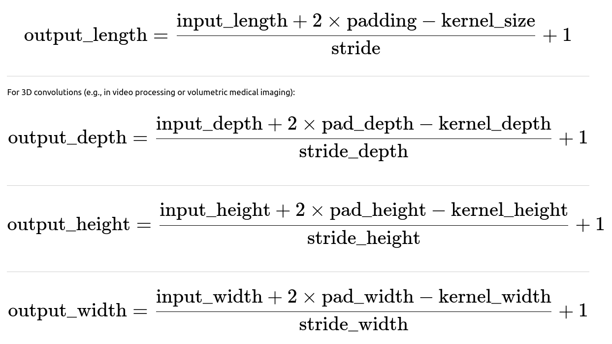
So it’s conceptually identical but extended to additional dimensions. A subtlety arises if your data has different sizes in each dimension (e.g., a video might have 16 frames in time, 128 in height, 128 in width). You must confirm that each dimension’s stride, kernel, and padding produce the correct final shape. Also, 3D convolutions can be extremely memory-heavy, so carefully selecting stride and kernel size is crucial to keep computations tractable.
How does data augmentation alter the effective input size for the convolution?
Many data augmentation techniques (like random crops, random scaling, or padding) can change the actual input size fed into the model. If you do random cropping to 28×28 on an original 32×32 image, you must ensure your convolution layers can still accept 28×28. Typically, if you use smaller or random input sizes, you rely on having enough padding or a design that can handle various shapes. A pitfall is forgetting that a random crop might produce shapes too small for certain layers. For instance, a network that expects at least 16×16 before a stride=2 downsampling might break if you feed it 8×8. Real-world data augmentation pipelines must be carefully tested so they do not produce invalid shapes.
How might a mismatch in the number of dimensions cause an error even if height and width are correct?
Convolutional layers expect input as (batch_size, channels, height, width) for 2D or (batch_size, channels, depth, height, width) for 3D. If you accidentally pass a tensor missing the channel dimension (like [batch_size, height, width]) or extra dimensions, you’ll see errors complaining about shape mismatch. This is not about the formula for calculating the spatial dimension but about ensuring the 4D or 5D input format is correct. Always confirm that the shape used for forward passes matches the layer’s expectations (e.g., for PyTorch Conv2d, you need 4D input). A subtle pitfall is having (batch_size=1) and then losing a dimension inadvertently, turning it into a 3D tensor.
In advanced segmentation tasks with large images, how do we handle memory constraints when computing the entire convolution at once?
Large images (e.g., 4K resolution) can lead to huge intermediate feature maps in memory when performing many channels or deeper layers. Even if the shape formula is correct, the memory might be insufficient. Common solutions:
Tiled inference: Split the large image into overlapping tiles, run the CNN on each tile, and then stitch the outputs. The shape formula applies locally per tile. The main pitfall is ensuring sufficient overlap to handle border effects so you don’t get segmentation artifacts at tile boundaries.
Reduced precision: Use mixed precision (float16) to shrink memory usage.
Checkpointing: Some frameworks allow gradient checkpointing to reduce memory usage at the cost of additional compute.
A subtlety is ensuring that when you stitch tiles, you maintain consistent results at the boundaries (e.g., reflection padding across tiles might differ from a single pass on the entire image). Debugging partial or repeated edges in the final output can be tricky.
When is pooling used instead of strided convolution, and how does that interplay with output dimension?
Many architectures use pooling (e.g., max or average) instead of a strided convolution to reduce spatial dimension. Pooling typically has its own kernel size, stride, and optional padding. For example, a 2×2 max pool with stride=2 halves the spatial dimension. The formula for a 2D pooling layer is analogous:

The subtlety is that strided convolutions can learn a downsampling filter, while pooling uses a fixed operation (like max or average). Some modern networks prefer strided convolutions for downsampling to keep everything “learnable,” while classic architectures (like VGG) use explicit pooling. In practice, you have to verify that each stage’s output dimension is consistent when mixing convolution layers (with or without stride) and pooling layers. A frequent pitfall is ignoring that the combination of consecutive pool layers might shrink the dimension more drastically than intended, especially if you use large stride in the convolution immediately afterward.