
ML Interview Q Series: Compare and contrast Gaussian Naive Bayes (GNB) and logistic regression as classification methods, and discuss the scenarios where one might be favored over the other.

📚 Browse the full ML Interview series here.
Short Compact solution
Both Gaussian Naive Bayes (GNB) and logistic regression are practical tools for classification tasks, with each offering particular advantages and disadvantages. GNB needs relatively fewer data points to achieve reasonable performance and can be fast to train, which proves helpful in situations where data are limited. Its results can also be interpreted easily in terms of estimated conditional probabilities. Logistic regression, on the other hand, is straightforward to interpret through class probabilities and allows analyzing how different input features influence the prediction.
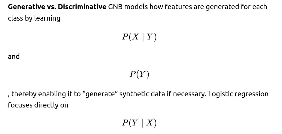
A key disadvantage of GNB is the assumption that all input features are conditionally independent, which often does not hold if the features are correlated. Meanwhile, logistic regression may fail to properly capture complex interactions between features if left in its basic form and can overfit when only minimal data are available. In terms of their fundamental differences, GNB functions as a generative classifier (modeling P(X∣Y) and P(Y)), while logistic regression is discriminative (directly modeling P(Y∣X)). Logistic regression typically relies on an optimization routine for learning, whereas GNB can leverage simple closed-form parameter estimates if its underlying assumptions are met. Both methods can yield linear decision boundaries and, under certain conditions, yield equivalent expressions for P(Y∣X).
When features exhibit correlation and there is an ample amount of data, logistic regression is often a better choice because it does not hinge on the conditional independence assumption. However, in domains with limited samples or strong prior knowledge about the data generation process, GNB can be advantageous due to its simplicity and efficiency in parameter estimation.
Comprehensive Explanation
Gaussian Naive Bayes (GNB) and logistic regression are both valuable classification strategies that often produce linear decision boundaries in feature space. Despite this similarity in how they partition the input space, the two models deviate in their conceptual approaches.
Underlying Model


Key Advantages
GNB
Learns effectively from fewer data points thanks to straightforward parameter estimation (e.g., using sample mean and variance for each class and feature).
Can be very fast at both training and inference due to its closed-form parameter updates.
Straightforward interpretability in terms of how each feature’s Gaussian distribution contributes to the posterior class probabilities.
Logistic Regression
Allows direct interpretation of feature coefficients and their impact on the log-odds of class membership.
Does not assume conditional independence among features, so it is typically more robust when features are correlated.
Flexible in practice: by introducing polynomial terms or domain-specific transformations of features, one can capture interactions or nonlinearities to some extent.
Principal Disadvantages
GNB
Relies on the assumption that features are conditionally independent given a class label. This assumption is frequently violated in real-world data containing correlated features.
If features depart significantly from normality, performance can degrade unless additional distributions or methods are used.
Logistic Regression
Basic logistic regression may not capture complex relationships between features unless additional feature-engineering or interaction terms are introduced.
Prone to overfitting when the number of features is large relative to the number of data points, although regularization techniques (like L2 or L1) can mitigate this.
Differences in Learning Approach
. In practice, discriminative methods often yield higher accuracy when there is an abundance of labeled data, because they do not commit modeling capacity to the joint distribution of features and labels.
Parameter Estimation Logistic regression estimates weights by solving an optimization (often via gradient descent or variants) that maximizes the conditional log-likelihood of labels given features. GNB can estimate parameters (means and variances of Gaussian distributions per class, plus class prior probabilities) in closed form using simple statistical formulas.
Similarities

When to Use GNB Over Logistic Regression
Whenever you have a very small dataset and strong assumptions about data distribution, GNB typically converges rapidly and can yield reliable results.
If you know the features are conditionally independent within each class, GNB’s assumptions hold, potentially making it very effective and simple to implement.
When to Use Logistic Regression Over GNB
When you expect important interactions between features or suspect high correlation among them. Logistic regression is more flexible in capturing these correlations (especially if feature transformations or regularization are applied).
When interpretability in terms of feature impact on class probabilities is important. The weights in logistic regression directly show how each feature contributes to the log-odds of the outcome.
Potential Follow-Up Question: Why Is Naive Bayes Called “Naive”?
Naive Bayes is “naive” because it treats each feature as being conditionally independent of every other feature, given the class label. In many practical datasets, features do exhibit correlations, so the naive conditional independence assumption is rarely strictly true. Nonetheless, Naive Bayes can still perform surprisingly well because parameter estimates can remain robust under partial violations of this assumption, especially in domains with limited data.
Potential Follow-Up Question: How Does Logistic Regression Handle Correlated Features Differently?

. If two features are correlated, logistic regression does not force their effects to be independent in modeling. Instead, it learns whichever weight combination best explains the observed labels. This flexibility often allows better performance in real-world scenarios where features are co-dependent, though it can require more data to estimate these interactions accurately.
Potential Follow-Up Question: Could GNB Outperform Logistic Regression Even With Enough Data?
Yes. If the data truly follow (or closely approximate) the conditional independence assumption and each feature’s distribution within a class is close to Gaussian, GNB can be extremely effective. In addition, if you have strong priors about the distribution of features given the class label, the Bayesian framework can leverage those priors. Logistic regression, if not regularized properly, could overfit or might require more data to accurately capture all relevant parameter values.
Potential Follow-Up Question: What Are Strategies to Avoid Overfitting in Logistic Regression?
Regularization is the primary mechanism. Commonly, one can introduce an L2 penalty (ridge regularization) or L1 penalty (lasso regularization) on the weight parameters. This ensures that coefficient magnitudes remain small, reducing variance in the model and enhancing generalization. Cross-validation is then used to select optimal hyperparameters (like the regularization strength).
Potential Follow-Up Question: How Would You Implement Logistic Regression and GNB in Python?
import numpy as np
from sklearn.linear_model import LogisticRegression
from sklearn.naive_bayes import GaussianNB
from sklearn.model_selection import train_test_split
from sklearn.metrics import accuracy_score

# Suppose X is your feature matrix and y is your label vector
X_train, X_test, y_train, y_test = train_test_split(X, y, test_size=0.2)

# Logistic Regression
log_reg_model = LogisticRegression()
log_reg_model.fit(X_train, y_train)
preds_log = log_reg_model.predict(X_test)
print("Logistic Regression Accuracy:", accuracy_score(y_test, preds_log))

# Gaussian Naive Bayes
gnb_model = GaussianNB()
gnb_model.fit(X_train, y_train)
preds_gnb = gnb_model.predict(X_test)
print("Gaussian Naive Bayes Accuracy:", accuracy_score(y_test, preds_gnb))
The above snippet uses scikit-learn, a widely adopted Python library for machine learning. LogisticRegression trains via an iterative optimization method (e.g., stochastic gradient descent internally), while GaussianNB estimates mean/variance for each class-feature combination and applies Bayes’ theorem at prediction time.
Potential Follow-Up Question: How to Address Class Imbalance in Logistic Regression and GNB?
Both methods can use specific techniques:
In logistic regression, class weights can be manually set or automatically computed by most libraries through the “class_weight” parameter. Also, oversampling the minority class (e.g., SMOTE) or undersampling the majority class can help.
For GNB, class priors can be adjusted or you can similarly perform resampling. If you have prior knowledge of different costs associated with misclassification, you can incorporate these costs into the prior probabilities of each class.
Below are additional follow-up questions
How would you handle continuous vs. discrete features in both GNB and logistic regression, and what are potential pitfalls if your data has a mixture of these feature types?
In Gaussian Naive Bayes, each numeric feature is typically assumed to follow a Gaussian (normal) distribution within each class. When encountering discrete or categorical features, GNB can either treat those as if they were continuous (which is often inappropriate and may violate the model’s assumptions), or use a different Naive Bayes variant (e.g., Bernoulli Naive Bayes for binary features or Multinomial Naive Bayes for count-based features). A potential pitfall is mixing numeric data in one distribution assumption and discrete data in another; if you do not carefully maintain separate conditional probability estimations for each feature type, the model might produce biased probability estimates.
Logistic regression can handle continuous or discrete input features as long as they are appropriately encoded (e.g., one-hot encoding for categorical variables). However, a subtle pitfall arises when you have high-cardinality categorical features, since expanding them into many dummy variables may result in excessive dimensionality, risking overfitting. Regularization (L2 or L1) can help mitigate this problem, but care must still be taken to avoid memory blow-up or extremely sparse matrices.
Another edge case is if a single categorical feature has multiple levels that rarely occur, or if some numeric features are highly skewed. In logistic regression, you may need transformations or grouping of rare categories; in GNB, you may need to properly model highly skewed numeric features using alternative distributions or carefully transform them into an approximate normal distribution before applying the Gaussian assumption.
What if the underlying distribution for some features in GNB is not actually Gaussian, and could that degrade performance?
GNB explicitly assumes each feature within a class follows a normal distribution. In reality, data might be skewed, multi-modal, or otherwise non-Gaussian. For instance, if you have data measuring time between events (often governed by an exponential distribution), simply applying GNB’s Gaussian assumption may lead to inaccurate estimates of P(X∣Y). Performance could degrade significantly in such mismatched situations.
A common workaround is to use alternative forms of Naive Bayes designed for the distribution at hand (e.g., Multinomial Naive Bayes for count-based text features, Bernoulli Naive Bayes for binary features, or kernel density estimates for continuous features that are not normal). Another approach is to apply data transformations to approximate normality (e.g., taking logarithms of positive, skewed data). Still, such transformations might complicate interpretability and require additional feature engineering effort.
How do these methods scale to multi-class classification, and are there significant differences in performance and interpretation?

independently. You simply compute posterior probabilities for each class and pick the one with the highest posterior. This process remains straightforward and typically requires minimal changes beyond storing more parameters (means and variances per class).
Logistic regression can handle multi-class scenarios in several ways:
One-vs-Rest (OvR), where the model trains one logistic regression per class to distinguish “this class vs. not this class.”
Softmax (multinomial) logistic regression, which extends the concept of log-odds to multiple classes simultaneously.
One potential pitfall with multi-class logistic regression is the complexity of the weight parameters. For example, in a K-class softmax logistic regression, you have parameters associated with each class in a single joint optimization. This can lead to more complex interactions among the parameter sets, potentially requiring more data and careful regularization.
When classes are imbalanced or numerous, GNB remains computationally efficient, but the conditional independence assumption might still hamper performance if features are correlated. Logistic regression in a multi-class setting might provide better calibrated probabilities but can require more careful hyperparameter tuning (e.g., regularization strength) for each class’s parameters.
How do both methods compare in real-time prediction scenarios with large-scale data, and what are potential memory or latency challenges?
Real-time or large-scale data processing often emphasizes minimal prediction latency, quick model updates, and memory efficiency:
GNB can be very quick in inference once parameters (means, variances, priors) are computed, as prediction merely requires evaluating Gaussian probabilities and multiplying them for each class. Parameter estimation is also straightforward to update incrementally if you keep running sums and sums of squares for the features. However, if you have numerous features or classes, storing separate mean and variance for each feature-class pair can become memory-intensive.
Logistic Regression typically evaluates a linear combination of features followed by a nonlinear activation (e.g., the sigmoid or softmax). Prediction is usually fast, but if your feature vector is extremely large (say, in high-dimensional text or image data), computing the dot product for each request might introduce latency constraints. If the model needs updating in real time, you must solve an optimization problem. Incremental or online learning versions of logistic regression exist (e.g., stochastic gradient descent), but they require careful tuning of the learning rate and regularization for stable convergence.
An edge case is when the data distribution drifts or changes abruptly over time. GNB can adapt if you have a mechanism to continuously recalculate means and variances. Logistic regression can adapt as well, but you must ensure the online optimization does not overfit new data points. In either approach, memory usage can become a bottleneck if you track too many historical observations or if your model is extremely large. Careful feature engineering, dimensionality reduction, or streaming algorithms can mitigate these issues.
What are some interpretability considerations when comparing GNB and logistic regression, especially for local vs. global explanations?
Both GNB and logistic regression can be considered relatively interpretable compared to more complex models like deep neural networks or random forests, but their interpretability differs:
GNB has a more “global” interpretability based on the per-class mean and variance of each feature. You can examine which features have the greatest separation in means across classes or where the variance is smallest. However, because of the conditional independence assumption, GNB does not directly capture interactions or correlations between features, so its explanations can be misleading if strong dependencies exist.
Logistic Regression has a clear “weight per feature” interpretation that contributes to the log-odds for a particular class (in binary classification) or among multiple classes (in softmax). This is often viewed as a simpler, direct measure of how each feature influences the outcome, assuming you have standardized or otherwise appropriately scaled your features. Nonetheless, if you have a large number of correlated features, interpreting individual weight coefficients can be tricky because each coefficient’s meaning depends on the other features in the model.
For local interpretability (explaining individual predictions), you can use tools like LIME or SHAP. However, logistic regression often yields a more coherent local explanation since the log-odds formula is straightforward to decompose. For GNB, local explanations might require visualizing how far a specific input is from each class’s mean in standardized units (e.g., Z-scores), but if features are correlated, this might be misleading.
What if some features have missing values or outliers, and how does this affect each model's assumptions and performance?
Missing Data:
GNB typically requires mean and variance for each feature-class combination. A naive approach is to drop instances with missing values or impute them. Dropping data reduces sample size, potentially undermining GNB’s advantage when data are already sparse. Imputation (e.g., mean imputation) can distort the variance estimate, especially if many values are missing. A pitfall is ignoring the correlation of missingness across features, which can degrade predictions.
Logistic regression also needs complete feature vectors unless imputation or some form of incomplete-data modeling is used. If your data have systematic missingness, logistic regression could produce biased estimates unless you carefully model or account for the missingness mechanism.
Outliers:
GNB’s Gaussian assumption is sensitive to outliers because they heavily affect the mean and variance calculations. A few extreme points can inflate variance and reduce the apparent discriminative power of a feature for that class. Proper outlier detection or robust measures (e.g., using truncated means) might be necessary.
Logistic regression can also be influenced by outliers, but if you employ regularization or robust estimation techniques, you can reduce the impact of extreme points. Nevertheless, large outliers in the feature space might shift the decision boundary significantly if not addressed.
Which hyperparameters typically need tuning for GNB and logistic regression, and how might one go about it?
GNB generally has fewer hyperparameters in its simplest Gaussian form. One might tune smoothing parameters (also known as “alpha” in certain implementations) that prevent zero probabilities. Smoothing can be crucial if certain features appear rarely. However, classical Gaussian Naive Bayes often uses the raw estimated means and variances without additional hyperparameters. This simplicity is part of its appeal, though it may limit flexibility.
Logistic Regression has multiple hyperparameters:
Regularization Strength: Often represented by “C” in many libraries, which is the inverse of regularization weight. Tuning it involves searching across different values to find a good balance between bias and variance.
Regularization Type: L1 (lasso), L2 (ridge), or elastic net. Each imposes different constraints on the coefficient structure. For instance, L1 can drive some coefficients to zero, aiding in feature selection. L2 tends to shrink all coefficients toward zero but not exactly to zero.
Solver: Libraries offer various solvers (e.g., “liblinear,” “saga,” or “lbfgs”). Depending on dataset size or sparsity, one solver might converge faster than another.
Cross-validation is commonly used to identify hyperparameters that yield the best performance metric (e.g., accuracy, F1, ROC AUC). One edge case is if you have an extremely small dataset, in which case exhaustive hyperparameter searches might lead to overfitting on the validation set. Carefully use nested cross-validation or Bayesian optimization to mitigate that risk.
How might one approach online or incremental learning scenarios, and do GNB and logistic regression adapt well to streaming data?
GNB can be made incremental by continually updating the means and variances of each feature for each class as new data arrives. You maintain running sums, sums of squares, and class counts. This approach allows GNB to handle streaming data with minimal overhead. However, if the data distribution starts changing drastically over time (concept drift), you may need a mechanism to “forget” or decay old statistics.
Logistic Regression can be adapted to an online context using stochastic gradient descent (SGD). Each new data sample (or mini-batch) updates the model weights. This approach, known as “online logistic regression” or “incremental logistic regression,” can handle extremely large data streams. A pitfall is selecting and tuning the learning rate schedule. If the rate is too high, the model might oscillate and fail to converge; if it’s too low, training can become very slow and may get stuck in poor local optima. Another edge case is abrupt shifts in data distribution, requiring dynamic adaptation or regular resetting of model parameters.
When might a parametric approach like GNB or logistic regression be insufficient, and how do we decide if a non-parametric method would be better?
Both GNB and logistic regression are parametric, meaning they assume a fixed functional form (e.g., linear decision boundary, Gaussian distribution of features in GNB). This can be too restrictive if:
The decision boundary is highly nonlinear or if there are complex, high-order interactions that are not captured by adding polynomial terms in logistic regression.
The distribution of features is distinctly non-Gaussian, multi-modal, or heavily skewed, making GNB’s assumption untenable.
The data are extremely large, and a more flexible method like random forests or gradient boosting might capture intricate patterns better.
You might consider non-parametric approaches (e.g., nearest neighbors, kernel methods, decision trees) if you have abundant data and suspect that the rigid assumptions of parametric models will lead to high bias. Yet, these non-parametric methods often require more memory and can be slower in inference (like KNN) or need more elaborate tuning (like random forests).
Pitfalls include:
Overfitting if you don’t have enough data relative to model capacity.
Interpretation challenges, since many non-parametric models lack the straightforward interpretability offered by logistic regression or GNB.
Potentially higher computational demands in training and/or prediction.