
ML Interview Q Series: Comparing Expected Values: Product of Two Dice Rolls vs. Square of One Roll
Browse all the Probability Interview Questions here.
4. There are two games involving dice that you can play. In the first game, you roll two die at once and get the dollar amount equivalent to the product of the rolls. In the second game, you roll one die and get the dollar amount equivalent to the square of that value. Which has the higher expected value and why?
When comparing the expected values of these two games, you want to determine which game, on average, yields a larger payout. These games both use fair six-sided dice (with faces numbered 1 through 6) but differ in how the payout is calculated. Here is a super detailed breakdown of the reasoning and the math involved, as well as potential follow-up questions that might arise in a rigorous interview setting.
Game 1: Two Dice, Payout is the Product of the Rolls
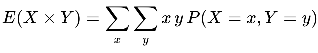
You roll two fair dice simultaneously (let’s call them die X and die Y). Each die independently takes values from 1 to 6 with equal probability of 1/6. The payout is X × Y. To find the expected value (mean) of this product:
We note that for two independent random variables X and Y, the expected value of their product is:

where X and Y are identically distributed discrete uniform random variables on {1, 2, 3, 4, 5, 6}. The expectation of a single fair six-sided die roll, E(X), is:


Therefore, the expected payout for Game 1 (two dice, product of rolls) is 12.25 dollars.
Alternatively, one could compute this without using the independence shortcut, by enumerating each possible product and averaging them. Either way, the result is 12.25.
Game 2: One Die, Payout is the Square of the Roll
In this game, you roll a single fair six-sided die (call it Z), and the payout is Z². To find the expected value:
We have:

Since each face has probability 1/6,
Hence, the expected payout for Game 2 is about 15.17 dollars.
Which Game Has the Higher Expected Value?
Comparing the two computed expectations:
Game 1 (product of two dice): 12.25
Game 2 (square of one die): 15.17 (approximately)
The second game has the higher expected value. Therefore, if you had to choose purely on the basis of expected value and both games cost the same to play, you would pick the second game (roll one die and square the result) to maximize your average winnings over many plays.
The reason behind this outcome is that squaring a single die roll grows values disproportionately at the higher end (e.g., 6² = 36 is quite large compared to 6 × 6 = 36, but because in the second game you always roll just one die, you only need to consider squares of [1..6], which yields an average that is higher than the mean product of two dice where smaller products like 1×1=1, 1×2=2, 2×2=4, etc. occur more frequently in the distribution of all possible products).
Below are some very thorough follow-up questions that might be asked in a high-level interview at a FANG company, along with deep, detailed explanations to each.
What is the distribution of outcomes for the product of two dice and for the square of one die, and how does that intuitively explain the difference in expected values?
For Game 1 (the product of two dice), the possible outcomes range from 1 (if both dice are 1) up to 36 (if both dice are 6). However, many mid-range products like 6, 8, 9, 10, 12, etc. appear quite frequently, while very high products like 36 require both dice to be 6, which is less probable (1/36).
For Game 2 (the square of a single die), the possible outcomes are 1, 4, 9, 16, 25, and 36. Each occurs with probability 1/6. Since these squares, especially 25 and 36, contribute heavily to the average and are not “diluted” by combinations leading to smaller products (like 2×3=6 or 1×5=5 in the first game), the expected value for squaring one die is higher overall.
Deeper Insight
In Game 1, every pair (x, y) with x, y ∈ {1..6} is equally likely (1/36). The product distribution skews toward moderate values, because there are many ways to obtain products like 6, 8, 10, 12, 15, 18, etc. but relatively fewer ways to get 36 (only one pair: (6,6)).
In Game 2, each square outcome {1, 4, 9, 16, 25, 36} is equally likely (1/6). High squares (25 and 36) occur more frequently in this distribution relative to the distribution of products for two dice. This “heavy tail” is what pushes the average payoff to be above 15.
Could you show a quick Python code snippet to empirically estimate these expectations by simulation?
Below is an example code you could run in a Python environment to empirically estimate the expected payouts. Such a simulation often helps confirm our theoretical derivations:
import random
import statistics

N = 10_000_000  # number of trials

# Game 1: Product of two dice
game1_results = []
for _ in range(N):
    die1 = random.randint(1, 6)
    die2 = random.randint(1, 6)
    game1_results.append(die1 * die2)

game1_avg = statistics.mean(game1_results)
print("Estimated Expected Value for Game 1 (Product of two dice):", game1_avg)

# Game 2: Square of one die
game2_results = []
for _ in range(N):
    die = random.randint(1, 6)
    game2_results.append(die * die)

game2_avg = statistics.mean(game2_results)
print("Estimated Expected Value for Game 2 (Square of one die):", game2_avg)
If you run this simulation for a large number of trials, you will see that:
game1_avgwill converge to around 12.25game2_avgwill converge to around 15.17
which matches our mathematical derivation.
Why does the formula E(X × Y) = E(X)E(Y) apply in this situation?
The key reason is that in Game 1, the two dice are independent. When two random variables X and Y are independent, the expected value of their product is the product of their expected values. Specifically:

Since rolling one die does not affect the outcome of rolling the other, X and Y are indeed independent, and so the formula holds.
What if the dice are not fair or if the rolls are not independent?
In real-world scenarios or certain puzzle setups, the dice might be biased, or the rolls might be somehow correlated. This can change the result:
Biased Dice: If the probability distribution for each face is different from 1/6, the expected value of a single die roll changes from 3.5 to something else. That immediately changes the product expectation.
Non-Independent Dice: If for some reason the outcome of the second die depends on the outcome of the first (for instance, conditional probabilities or a strange physical constraint), then you cannot simply multiply the means to get E(X×Y). Instead, you would need the full distribution or the correlation structure of the two dice to compute the expected product.
However, under normal assumptions (fair, independent dice), E(X×Y) = E(X)E(Y) = 12.25.
How does variance come into play for these two games, and can that be relevant?
While the question only focuses on expected values, sometimes interviewers push for deeper insights, including variance and risk analysis.
Variance for the product of two dice (Game 1): The random variable is X×Y. The variance can be computed if you know E((X×Y)²) and E(X×Y). However, the distribution is somewhat more complicated.
Variance for the square of one die (Game 2): Variance can be computed if you know E(Z²²) = E(Z⁴) and E(Z²).
In some decision-making settings, especially if the game were played once with high stakes, a person might prefer a less volatile game with a slightly lower mean over a more volatile game with a higher mean. But typically, with enough repetitions and no additional risk constraints, the game with the higher expected value is preferred. In this particular question, the second game not only has a higher expected value but the comparison is straightforward enough that you usually pick Game 2.
What if an interviewer asks about enumerating all possible outcomes for the first game explicitly?
You could list all pairs (x, y) where x and y range from 1 to 6, compute x×y for each pair, and then average. The total number of pairs is 36. Each has probability 1/36. The sum of products for all 36 pairs is:
1×1 + 1×2 + ... + 1×6 2×1 + 2×2 + ... + 2×6 ... 6×1 + 6×2 + ... + 6×6
One can systematically compute or quickly see:
The sum of 1×(1..6) is 1+2+3+4+5+6 = 21
The sum of 2×(1..6) is 2+4+6+8+10+12 = 42
And so on...
If you sum all these lines and then divide by 36, you will get 12.25. It’s more tedious, but it confirms the simpler approach E(X) × E(Y).
Could you talk about the practical significance of such expected value questions in real interview scenarios?
Often, a FANG-type interview question about dice or other random processes aims to see if a candidate:
Understands the definition of expected value.
Can identify when random variables are independent (and use the E(X×Y)=E(X)E(Y) property).
Knows basic sums of squares or other fundamental arithmetic series.
Thinks carefully about enumerating possibilities or employing direct probability-based formulas.
Such questions probe both conceptual depth (knowing independence) and comfort with elementary probability calculations (like E(X), E(X²), E(XY)). If you are strong in probability theory, you can easily manipulate these expectations and also confidently discuss generalizations (e.g., correlations, different distributions, advanced expansions).
Could the difference in expected values be further explained by the fact that squaring “magnifies” higher rolls more than multiplying two separate dice?
Yes, exactly. Squaring a single high number (like 6 → 36) is a fairly large jump from its baseline 6. Meanwhile, in the product scenario, to get 36 you need 6 on both dice simultaneously, which is less probable (1/36 chance). The shape of the distribution is quite important:
In Game 2, 36 occurs 1 out of every 6 rolls on average (probability = 1/6) because you only need a single 6.
In Game 1, 36 occurs 1 out of every 36 pairs on average (probability = 1/36).
That difference in how frequently high numbers can appear is a key driver of the difference in means.
Why might this question be considered tricky in an interview?
Some candidates might quickly guess that rolling two dice and multiplying might lead to a larger payoff because “two dice can get bigger numbers in more ways.” However, the presence of smaller possible products (such as 1×2=2, 1×1=1, 2×2=4, etc.) and the relatively low probability of both dice being large at the same time bring the average down compared to the squaring approach. This is often a “trap” to see if the candidate actually calculates the expected values properly rather than guessing incorrectly.
In a real betting scenario, how should we choose?
If both games cost the same to enter and there are no other constraints, you should choose the game with the higher expected value. In this case, Game 2 (the single die squared) has an expected payout of about 15.17, which exceeds 12.25 from Game 1, so Game 2 is superior in terms of average return.
What if there was a difference in cost or if we repeated the game multiple times?
If the cost of playing each game was different: Suppose Game 1 costs $C1 and Game 2 costs $C2. You’d compare E1 − C1 vs. E2 − C2. If (E2 − C2) > (E1 − C1), then you pick Game 2, and vice versa. It’s all about net expected profit after costs.
If you repeat the game many times: Typically, the Law of Large Numbers indicates the average payoff per play converges to the theoretical expected value. Over the long run, a higher expected value yields higher total earnings.
Could you consider the median or mode instead of the mean for decision making?
Sometimes, especially in risk-averse strategies or specific contexts, one might look at other metrics like the median or the mode of the payout distribution.
For Game 1, the mode of the product might be among values like 6 or 12 (because there are multiple ways to get those products), so the mode might be near that range.
For Game 2, each square {1, 4, 9, 16, 25, 36} is equally likely, so there is no single mode—each has probability 1/6.
However, the question explicitly focuses on expected value, which is the standard measure for average outcomes over repeated trials.
Do these results change if we use more dice or a different transformation?
More Dice: If you multiply more dice, or consider higher powers, the analysis changes and you need to recalculate the expectation based on the new setup. As the number of dice grows, certain transformations might have interesting properties (for instance, the sum of dice approximates a normal distribution for large counts, but product or squares have different behaviors).
Different Transformation: If, for example, you took the cube of one die vs. the product of three dice, you’d have a new set of expected values to compare. In general, for any random variable X, transformations like X², X³, e^X, etc., can drastically shift the distribution. You evaluate each on a case-by-case basis.
Final Answer to the Original Question
Between the two games:
Game 1 (two dice, product) has an expected value of 12.25.
Game 2 (one die, square) has an expected value of about 15.17.
Therefore, Game 2 has the higher expected value. The intuitive reason is that squaring a single die roll consistently yields a high average, especially because 6² = 36 occurs with probability 1/6, whereas in the product game, 36 only occurs with probability 1/36.
Below are additional follow-up questions
What if the dice are not standard six-sided dice (e.g., custom dice with faces 1 to N) for each game, and how do we compare expected values in that scenario?
When the dice faces extend from 1 to N instead of 1 to 6, the overall structure of each game remains the same, but the expected values change. Let’s define:
Game 1 (Modified): Roll two identical dice with faces {1, 2, ..., N}. The payout is the product of the two outcomes, X and Y.
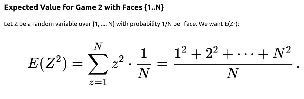
Game 2 (Modified): Roll a single die with faces {1, 2, ..., N}. The payout is the square of the outcome Z.
Expected Value for Game 1 with Faces {1..N}
Let X and Y be independent, identically distributed uniform random variables over {1, ..., N}, each with probability 1/N per face. The expected payout:

because X and Y are independent and identically distributed. For a single N-sided fair die,


Comparison


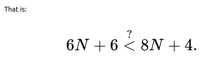
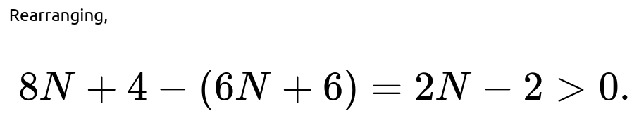
Hence, for N > 1, indeed E_2(N) > E_1(N). The only corner cases are:
N=1, in which case both games yield 1 (the product or the square is always 1), so E_1=E_2=1.
For any N > 1, squaring the single die yields a higher expected value than multiplying two dice.
Potential Pitfalls
If the dice are not fair but still have faces {1..N}, the distribution changes. You must carefully compute E(X), E(X²), etc., using the actual probabilities rather than the simple uniform formula.
If N is extremely large, the difference in expected values grows. The ratio E_2(N)/E_1(N) changes as N increases, and it typically remains >1 for N≥2.
How do payout caps or limits to winnings affect which game is better if a maximum payout is imposed?
Scenario Description
Suppose there is a rule that says, “You cannot earn more than M dollars on any single roll.” This cap M modifies the payout distribution by truncating or clamping the raw outcome.
Impact on Game 1 (Product of Two Dice)
If the product is X×Y, but we have a cap M, the actual payout is:

For standard dice, the maximum product is 36. If M < 36, then your winning is truncated to M whenever the product exceeds M. For instance, if M=20, any product above 20 becomes 20.
Impact on Game 2 (Square of One Die)
Similarly, the actual payout is:

The maximum square is 36 for a standard six-sided die. If M < 36, then any squared result that exceeds M gets capped at M.
Analytical Consequences
Truncating or clamping reduces the upper tail of the distribution. Since the second game relies heavily on the value 36 to pull its average upward, capping the payout might have a more substantial effect on Game 2’s average than on Game 1’s average (because 36 occurs with probability 1/6, making that big tail beneficial; if you reduce 36 to M, you lose a significant chunk of expected payoff if M < 36).
Conversely, in Game 1, the product 36 occurs with probability 1/36, so capping that at M might not drastically reduce the expected value (although it still reduces it somewhat). The question is whether the second game remains superior after imposing M. You’d need to compute the new truncated expectations:
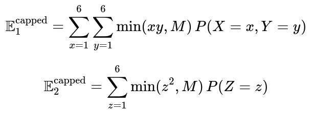
where each basic probability is 1/36 for the first game and 1/6 for the second. Depending on how large or small M is, it could reverse which game has the higher effective average payout.
Potential Pitfalls
Overlooking that capping might change the ranking of the two games if M is relatively low.
Failing to compute the new truncated distributions carefully: you must systematically account for how often each outcome exceeds M and clamp accordingly.
What if the game had a payoff that is a function of both the sum and the product of the dice? How does that compare to the square of a single die?
Consider a hypothetical variation: “Game 3: Roll two dice X and Y. Your payout is f(X, Y) = (X + Y) + (X×Y).” This merges a linear term (the sum) with a multiplicative term (the product). We might wonder how to compute the expected value and see if it surpasses the square-based game.
Computation
For two fair, independent six-sided dice:

This would actually exceed 15.17, the expectation for Z² (where Z is a single die). So if such a new combined function were offered, it might have an even higher expected value. This demonstrates how combining operations can drastically shift the mean.
Subtlety
Why is this relevant? In an interview, the question might shift to see whether you understand how sums and products of random variables can be combined. This question also hints that carefully analyzing transformations or combinations can result in surprising results (like an even bigger payoff than the square game).
Potential Pitfalls
Mistaking that you need to do a full enumerated sum for f(X, Y). You can do that, but using the linearity of expectation and independence properties often simplifies it significantly.
Forgetting that the expected value of a sum is the sum of expected values, so you can break it down into smaller, easier parts.
How does the concept of higher-order moments (e.g., skewness or kurtosis) differ between these two games, and why might that matter in certain real-world contexts?
Although the interview question focuses on the expected value, some real-world applications (e.g., finance, insurance, risk management) care about distribution shape, not just the mean.
Skewness and Kurtosis
Skewness measures the asymmetry of the distribution.
Kurtosis measures the “tailedness,” or how heavy the tails are compared to a normal distribution.
For Game 1 (Product of X and Y), the distribution might be more peaked around moderate values (e.g., 6, 8, 12, 18) with relatively fewer occurrences of 36. For Game 2 (Z²), you have discrete outcomes {1, 4, 9, 16, 25, 36} each with probability 1/6, so it’s not as heavily “peaked” around the center—each outcome is equally likely.
Real-World Implications
A distribution with higher kurtosis might mean more extreme outliers. If you are a risk-averse player, you might prefer a distribution with fewer large outliers (even if the mean is high).
In some contexts, having more consistency (a narrower distribution) might be beneficial if you can’t absorb large fluctuations.
Potential Pitfalls
Failing to realize that just because one game has a higher expected value, it might also have a higher variance or heavier tails (or, conversely, missing that if you wanted stable returns, you might pick a game with a lower standard deviation).
Confusion of average with the entire distribution shape can lead to misinformed decisions if the scenario involves risk constraints.
If you could see the result of the first die in Game 1 before choosing to multiply by a second die or opt out, could you change your expected winnings?
Imagine a variation:
You roll one die first and observe its outcome X.
You can choose to either “accept the product game” by rolling a second die Y and taking X×Y, or you can choose a fallback payout (like $0 or some known amount).
Is there a strategy that improves your expected payout?
Analysis
Assume the fallback is $0 for simplicity. Let X be the observed outcome of the first die. The expected value of rolling the second die if you choose to proceed is:

Thus, if x is your first die, the expected product is 3.5x. If you decide that you either proceed or get $0, the best strategy is to always proceed for x>0 (which is always true for a standard die). You always improve your expected payoff by rolling the second die. Hence you gain no strategic advantage in “opting out,” because x≥1 and 3.5×1=3.5 is better than 0.
Could You Choose Between Games?
Another interesting scenario is: after seeing the first die in Game 1, you get to choose between finishing Game 1 or switching to Game 2 (some hypothetical scenario). This might alter the decision if Game 2’s outcome is still unknown. However, typically, you’re not allowed such free switching after partial information. But if an interviewer suggests it, you’d have to compute expected values for each game conditionally.
Potential Pitfalls
Overthinking the partial information aspect if the fallback is always worse.
Forgetting that the expected outcome from continuing to multiply by a second die is linear in x, so any positive x is beneficial to continue playing rather than forfeiting.
What about player psychology or utility theory (e.g., diminishing returns for large payouts)? Does that change which game one might prefer?
In expected utility theory, a player’s objective might not be to maximize the raw dollar expected value, but to maximize the expected utility of the payoff. A classic example is a concave utility function, such as:

When you have a concave utility, large amounts are “less valuable” than linear scaling would suggest, reflecting risk aversion.
Applying Utility to Game 1 vs. Game 2
Game 1: The payout is X×Y, so the utility is something like U(X×Y).
Game 2: The payout is Z², so the utility is U(Z²).
You’d need to compute:

and compare them. The result can differ from which game has a higher raw expected value. For example, a game with frequent moderate payoffs might yield a higher expected utility for risk-averse players than a game with a higher but more volatile payoff.
Potential Pitfalls
Assuming the game with the highest expected monetary value automatically has the highest expected utility. This is only true under a linear utility function.
Overlooking that humans (or real players) often exhibit risk aversion or risk-seeking behavior, potentially reversing the preference indicated by the simple expected value criterion.
How would results differ if the dice had faces labeled with negative numbers or a mixture of positive and negative numbers?
Suppose you have a custom die with faces {−3, −2, −1, 0, 1, 2} or some other combination. This changes everything:
Game 1: The product X×Y can be negative, zero, or positive. If both dice are negative, you get a positive product; if one is negative and the other positive, you get a negative product; if either is zero, the product is zero. You must carefully calculate probabilities of each outcome.
Game 2: If you square the single die’s outcome, negative values become positive. For example, (−2)²=4 is the same as 2²=4. This might drastically change the distribution, possibly leading to a higher average than the product game if negative or zero faces are involved.
Analyzing a Simple Example
Let’s define a hypothetical 6-sided die with faces {−1, −1, 0, 1, 1, 2} just as an example:
Game 1: Payout = X×Y. You’d need to list the possible pairs, compute each product, multiply by their probabilities, and get E(X×Y).
Game 2: Payout = Z². You’d compute E(Z²) by summing squares of each face times 1/6.
It might turn out that squaring a single random face yields a certain positive average, while the product distribution for two such dice could be less straightforward—some negative products, some zero, some positive. The relative performance depends on the particular labeling of the die.
Potential Pitfalls
Failing to realize that negative or zero faces can shift the entire distribution and might cause the product-based game to have a lower or even negative expected value.
Missing that squaring negative numbers yields positive payoffs, which can drastically inflate the square-based game’s average payoff relative to the product game.
In a practical coding interview, how might you handle large simulations for these games efficiently?
Memory and Computation Considerations
Simulation Size: If you want to reduce the variance of your Monte Carlo estimates, you might run tens of millions of trials. That can be time-consuming. You need to use efficient random number generation and avoid unnecessary overhead in the loop.
Vectorized Approaches: In Python, one approach is to use NumPy for vectorized operations. For instance:
import numpy as np

N = 10_000_000
rolls_1 = np.random.randint(1, 7, size=N)
rolls_2 = np.random.randint(1, 7, size=N)
products = rolls_1 * rolls_2
expected_product = np.mean(products)

rolls_3 = np.random.randint(1, 7, size=N)
squares = rolls_3 ** 2
expected_square = np.mean(squares)
Vectorization is much faster than pure Python loops, especially at large N.
Potential Pitfalls
Using random.randint in a pure Python loop of 10 million iterations might be too slow. NumPy’s vectorized operations are typically more efficient.
Not using a fixed seed if you want reproducible results. Usually, for an interview or demonstration, you might fix the seed:
np.random.seed(42)
to show consistent results.
If memory is constrained, you might generate the data in chunks instead of all at once.
What if a candidate tries to guess the answer without computing, incorrectly claiming the product game must have a higher payout “since it uses two dice?” How should one respond?
This is a common misconception. One might think that more dice or more complicated operations automatically produce a bigger average. The correct approach is:

Intuitive explanation: Highlight how a single 6 in the square game yields 36 with probability 1/6, while 36 in the product game requires both dice to be 6 with probability 1/36.
Potential Pitfalls
Accepting “intuitive” arguments without verifying through actual expectation calculations.
Underestimating how powerful squaring a single high roll can be.
How could rounding or integer constraints alter the expected values in an implementation?
In some real systems, perhaps the payout must be an integer, or the roll might be read from an integer sensor with some error. Usually, dice are discrete anyway, so that’s not a big difference. But if you had to apply special rounding rules to the final result, that can shift the expectation slightly.
For example, if you always round down to the nearest multiple of 5, then you’d recalculate:
For Game 1: Payout = floor(5 * round((X×Y)/5)) or something similar.
For Game 2: Payout = floor(5 * round(Z² / 5)).
You would need to systematically account for that transformation:

Rounding inside the expectation and taking the expectation after rounding are not the same. This might reduce the difference between the two games or shift which game is preferred.
Potential Pitfalls
Incorrectly applying rounding to the average rather than to individual outcomes.
Missing that floor or rounding transformations can significantly change expected values because the operation is nonlinear.
How might confidence intervals or statistical significance be addressed if we only have a limited number of actual dice rolls?
If you’re running a real experiment with a small number of trials, your sample average for each game might deviate from the theoretical mean. You could construct a confidence interval for each game’s average payoff:
For Game 1, gather n products from n pairs of dice rolls, compute the sample mean and sample variance, and use standard formulas for a confidence interval:

is the appropriate value from the normal distribution for the confidence level you want.
For Game 2, similarly, gather n squares from n single-die rolls, compute the sample mean, sample variance, and the same type of confidence interval.

You would only conclude that one game has a higher expected payout if their confidence intervals don’t overlap sufficiently—or more precisely, if the difference in sample means is significantly greater than zero by a standard hypothesis test. With enough rolls, you can be quite confident that Game 2 surpasses Game 1.
Potential Pitfalls
Using too few rolls, leading to wide confidence intervals that overlap and fail to show a difference in means.
Misapplying the normal approximation for small sample sizes, or ignoring that the distribution is discrete.
Could we design an alternative game where the expected values are equal?
Yes, you can tweak the transformation on a single die until it matches 12.25. Suppose we define “Game 3” with a payout of
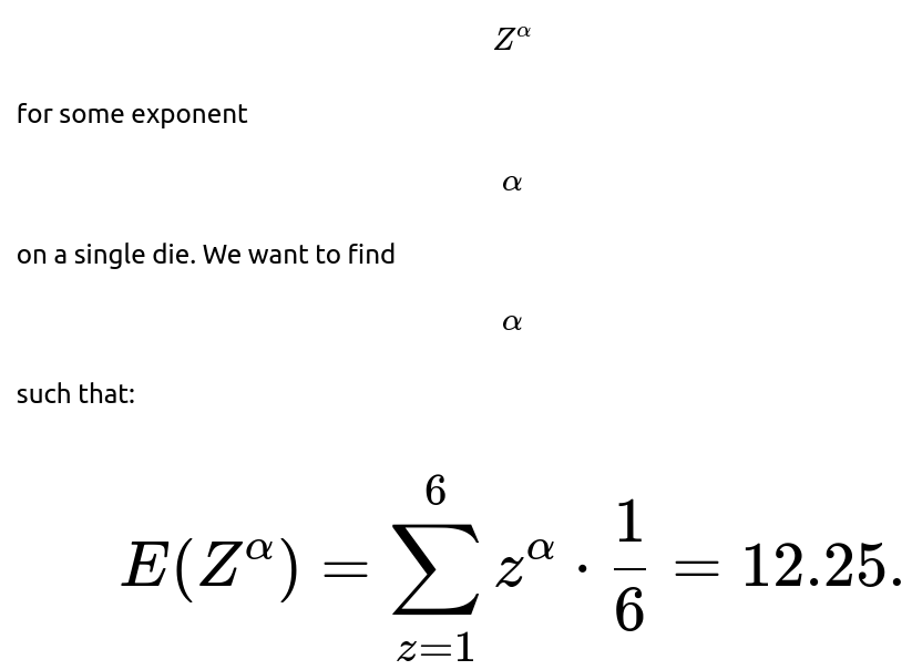

, we might find an exponent somewhere between 1 and 2 that produces an expectation of 12.25. This is more of a curiosity but highlights the idea that the shape of the function that transforms the die roll strongly affects the average.
Potential Pitfalls
Getting stuck trying to solve

analytically; it’s often easiest to do a small numerical search in code.
Forgetting that even if you match the means, the distribution shape (variance, skewness, etc.) might still differ.

How does knowledge of independence and the linearity of expectation generalize to more complex dice or more general random variables?
When random variables are independent:
provided X_1 and X_2 are independent.
For the dice scenario, it’s straightforward, but if you have correlated dice or special physical constraints, you can’t just multiply their means to get the mean of the product. Instead, you’d need:
The same principles apply if you have more dice or a complicated joint distribution. If an interviewer extends the question to, say, rolling multiple dice with unusual correlation structures, your ability to compute or approximate the expectation depends on enumerating or sampling from the joint distribution.
Potential Pitfalls
Assuming independence in a scenario with hidden correlations (e.g., loaded dice that correlate your second roll with the first).
Failing to see that linearity of expectation still holds for sums even if the variables are not independent, but for the product, you specifically need independence.
If the die was continuously distributed over an interval (e.g., from 1 to 6 in a uniform continuous manner), how would that compare?
Though a standard “die” is discrete, an interviewer might ask a hypothetical: “Assume we have a random variable uniformly distributed over [1, 6]. Then compare X×Y vs. Z² for a single random variable in [1, 6].”
Continuous Case
For X, Y ∼ Uniform(1, 6), we compute:


That’s a bit lower than the discrete case’s 15.17 for squares, but it’s still higher than 12.25 for the continuous product distribution. The difference arises because the integrals of squares over [1,6] differ from the discrete sums for {1,2,3,4,5,6}, but the pattern (square vs. product) remains the same in terms of which is bigger.
Potential Pitfalls
Confusing the discrete case’s sum-of-squares formula with the continuous integral.
Forgetting that even though the uniform distribution’s mean is the same as the discrete distribution, the second moment can differ.
How might using these dice games in an interview test knowledge beyond probability?
Interviewers might want to see:
Coding Skills: The candidate’s ability to implement a quick simulation in Python and verify results.
Statistical Reasoning: Comfort with expected values, independence, distributions, and transformations.
Communication: Explaining why a single die squared can beat two dice multiplied, particularly if the “intuitive guess” is reversed.
Generalization: The ability to extend or modify the approach to new distributions or transformations (sums, products, squares, logs, etc.).
Creativity: Proposing new game structures or alternative payoffs, or applying risk analysis to decide among them.
Each of these aspects might be probed in different ways by follow-up questions that have little to do with dice per se but test underlying problem-solving skills and theoretical knowledge.
How can floating-point precision issues arise in large-scale simulations, and are they relevant here?
In Python or other languages, floating-point arithmetic can cause small rounding errors. For dice-based computations, because all sums are typically small integers or short sums of integers, you won’t see massive floating-point issues. However, if:
You do extremely large number of trials (e.g., hundreds of millions) in a simulation,
You have dice that produce very large values (like dice up to 100,000),
You repeatedly add or multiply many values,
then floating-point precision might accumulate errors. Mitigations include using double precision (default in Python’s float) or specialized libraries for arbitrary-precision arithmetic if truly needed.
Potential Pitfalls
Overly trusting that floating-point arithmetic will never matter. Usually for typical dice games, the effect is negligible, but in large-scale or special transformations, it might become relevant.
Attempting to store enormous intermediate products (e.g., 100,000 × 100,000) could exceed normal integer or float bounds in some languages (less of an issue in Python since it has long int, but still relevant for floating-point rounding).
How do sampling errors in real dice rolling compare to the ideal theoretical model?
Real dice may not be perfectly balanced, and physical rolls can be biased or might not reflect purely random processes. Additionally:
Repeated rolling by hand can cause correlation if the person’s rolling technique is systematically biased.
The sample size in practical testing might be limited.
Still, for most casual or typical “fair dice” assumptions, these biases are minimal. But if an interviewer wants to see if you’re aware of real-world subtleties, you might mention:
Empirical Testing: Gather data from actual dice rolls, run a chi-squared test to check for face fairness.
Systematic Deviation: If the dice are heavier on one side, the distribution changes, so the expected values may deviate from 12.25 or 15.17.
Mitigation: Rolling in a dice tower or using automated dice rollers to reduce repeated patterns.
Potential Pitfalls
Overlooking real-world biases and assuming purely theoretical results apply exactly without acknowledging physical imperfections.
Not clarifying that in typical puzzle or interview contexts, “fair dice” is a standard assumption.
How could a dynamic programming or state-based approach be applied if the games were multi-stage?
If the dice game were extended into multiple stages—say you have multiple rolls that accumulate a product, or you have an “option to keep rolling or stop”—you might use dynamic programming (DP) to find the optimal strategy. For example:
If in each turn you can choose to stop and collect your current product or roll again and multiply by a new die result, what’s the maximum expected final product?
If the second game let you re-roll a certain number of times and take the best square out of your attempts, that changes the distribution further.
Such multi-stage expansions go beyond the simple one-roll scenario but illustrate how you’d:
Define states (e.g., how many rolls left, current partial product).
Compute expected transitions from each state.
Use backward induction to find an optimal stopping or continuing rule that maximizes expected payout.
Potential Pitfalls
Failing to properly define the state space or transition probabilities.
Not realizing that as soon as you have a “stop or continue” choice, the problem is no longer trivial and often must be solved by enumerating possible outcomes or using DP or other search methods.
How might Markov Chain techniques or advanced probability approaches become relevant?
In single-shot dice games, Markov Chains are not particularly relevant. But if you have repeated rolling with memory (states based on previous outcomes), you may model it as a Markov Chain. For instance:
A game where the payout depends on the product of consecutive rolls over time.
A game that ends when a certain condition is met (e.g., rolling doubles or achieving a certain sum).
In these extended scenarios, you’d set up a Markov Chain with states that track the needed information (like the last roll or partial total) and transition probabilities. Then you could compute the expected total payout or the probability of eventually hitting some event. This is advanced but demonstrates broader mastery of probability theory.
Potential Pitfalls
Trying to apply Markov Chains to a single roll situation unnecessarily, which can overcomplicate the problem.
Misidentifying the state representation if the game’s payoff depends on multiple previous rolls.

