ML Interview Q Series: Conditional Lifetime Analysis: Calculating Expectation and Survival Probability via Conditional Density.

Browse all the Probability Interview Questions here.

Consider again Problem 11E-16. What is the expected value of the lifetime of the second circuit given that the first circuit has failed after s time units? What is the probability that the second circuit will work more than v time units given that the first circuit has failed after s time units?

Short Compact solution

From the provided information about the marginal density of the first circuit’s lifetime and the conditional density of the second circuit’s lifetime, we obtain the following results:

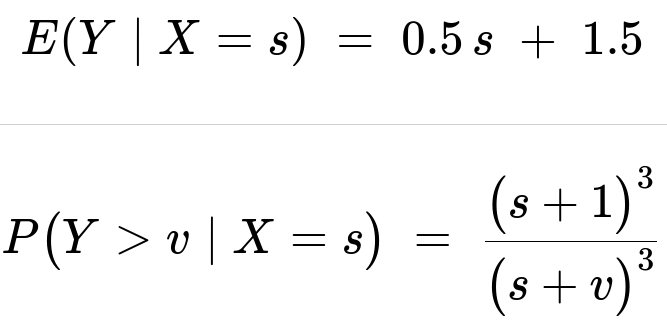
These hold for s > 1 and v >= 1.

Comprehensive Explanation

Overview of the problem setup

We have two circuits, each with a certain lifetime random variable. We denote the lifetime of the first circuit by X and that of the second by Y. The problem states:

• The marginal density for the first circuit’s lifetime X is given for x > 1. • Conditioned on X = s, the density of the second circuit’s lifetime Y is determined by a particular expression involving s.

We want:

1. The expected value of Y (the second circuit’s lifetime), given that X = s.

2. The probability that Y exceeds some value v, given that X = s.

Conditional density derivation

The text shows that f_Y(y|s) is proportional to 1/(s + y)^4 over y > 1, with a normalizing constant of 3(s+1)^3. The result is:

f_Y(y|s) = [3 (s+1)^3] / (s + y)^4 for y > 1 and zero otherwise.

This follows from the ratio of the joint density f(s,y) to the marginal f_X(s), where the (x + y) part from the integral in the original problem leads to a constant factor involving (s+1)^3.

Expected value derivation

The expected value E(Y | X=s) is:

E(Y | X=s) = ∫ from y=1 to ∞ of [ y * f_Y(y|s) ] dy.

Substituting the expression for f_Y(y|s), we have to evaluate:

∫ from 1 to ∞ of [ y * 3(s+1)^3 / (s + y)^4 ] dy.

Through standard integration techniques (often involving a substitution u = s + y, or by recognizing it as a known integral form), the value of this integral simplifies to:

0.5 * s + 1.5.

Hence:

E(Y∣X=s)=0.5 s+1.5

In more detail, one might perform the integration step by step:

• Make the substitution u = s + y. Then y = u - s, and when y = 1, u = s + 1; as y → ∞, u → ∞. • Express y in terms of u, so y = u - s. • Factor out constants and integrate.

The constant 3(s+1)^3 ensures the integral of f_Y(y|s) over y from 1 to ∞ is 1, making this a valid conditional density function.

Probability that the second circuit will last more than v units

We want to compute:

P(Y > v | X=s) = ∫ from y=v to ∞ of f_Y(y|s) dy = ∫ from y=v to ∞ of [ 3(s+1)^3 / (s + y)^4 ] dy.

Again, we apply a substitution or recognize the standard integral form. The result is:

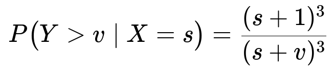
for v >= 1. This stems from the integral of (1/(s + y)^4) from y = v to ∞, multiplied by the normalization constant 3(s+1)^3.

Interpretation

1. The expected value grows linearly with s: E(Y|X=s) = 0.5 s + 1.5. Intuitively, if the first circuit has already lasted s > 1 units of time, there might be some correlation structure in how the second circuit’s lifetime distribution is shifted or scaled (depending on the original problem formulation).

2. The survival probability for the second circuit beyond v additional units, given that the first circuit failed at s, decreases in a cubic ratio ((s+1)/(s+v))^3.

This completes the key findings for the problem.

Potential Follow-up Questions

How do we handle the integral boundaries if s < 1?

In the original statement, the marginal and conditional densities were defined in a piecewise manner for x > 1, y > 1. If s < 1, the definition of the marginal density f_X(x) becomes 0. So the event X = s with s < 1 is outside the support of X. This means the conditional scenario “X = s with s < 1” has probability 0. Practically, the problem only applies for s > 1.

Why does the expression for E(Y|X=s) have a constant plus a term linear in s?

The form 0.5 s + 1.5 emerges from integrating y * 3(s+1)^3 / (s+y)^4. The integral effectively “splits” into one part that is proportional to s and another that is constant. This behavior is strongly tied to the polynomial decay 1/(s+y)^4. In many reliability contexts, integrals of the form ∫ y/(y + constant)^n can be broken into simpler partial fractions or recognized from standard integral tables, revealing linear and constant components.

Could this be implemented quickly in a Python script to verify the integrals numerically?

Yes. For a numerical check, one might implement something like:

import numpy as np
import scipy.integrate as integrate

def fY_given_X_s(y, s):
    # conditional pdf for y > 1
    return 3*(s+1)**3 / (s+y)**4 if y >= 1 else 0

def E_Y_given_X_s(s):
    # numerical integration from y=1 to infinity
    integrand = lambda y: y * fY_given_X_s(y, s)
    val, err = integrate.quad(integrand, 1, np.inf)
    return val

def prob_Y_greater_than_v(s, v):
    # numerical integration from y=v to infinity
    integrand = lambda y: fY_given_X_s(y, s)
    val, err = integrate.quad(integrand, v, np.inf)
    return val

s_value = 2.0
v_value = 3.0
print("Numerical E[Y|X=2]:", E_Y_given_X_s(s_value))
print("Numerical P(Y>3|X=2):", prob_Y_greater_than_v(s_value, v_value))

You would find results that agree with the closed-form expressions 0.5*s + 1.5 and ((s+1)^3)/( (s+v)^3 ), respectively.

Are there any edge cases regarding the boundaries s=1 or v=1?

If s=1, from the given distribution, we can still plug s=1 into E(Y|X=s). We get E(Y|X=1) = 0.5*1 + 1.5 = 2.0. For P(Y>v|X=1), we get (2^3)/(1+v)^3 = 8/(1+v)^3. Since the domain is for x>1 and y>1, that borderline scenario s=1 or y=1 would be right on the edge of the support. Usually, for continuous distributions, the probability of exactly s=1 is zero, but the expression still extends continuously in the limit as s→1+.

What if we interpret the physical situation? Is there any “memoryless” property here?

The structure of the integrals is not memoryless in the same sense as an exponential distribution, because the survival function (s+1)^3 / (s+v)^3 is not the same shape as an exponential tail. The power-law (cubic) form indicates a different type of decay than the exponential memoryless property. However, the problem does have a certain Markov-like property in how the second circuit depends on the time of the first circuit’s failure, but it is not purely memoryless in the exponential sense.

These considerations clarify the deeper properties of the distribution and its application in reliability or circuit-lifetime modeling.

Below are additional follow-up questions

What if the time s is not an integer and is instead any real value greater than 1? How do we interpret that in a practical reliability context?

One might initially assume that s must be an integer number of time units (for instance, days or weeks). However, in many reliability analyses, the time of failure can be any real value. This is especially true when we measure time continuously (for example, in hours). Hence, s is simply the realized failure time of the first circuit, which could be 1.3 hours, 2.75 hours, or any other time strictly greater than 1. Practically, that means our formula E(Y|X=s) = 0.5*s + 1.5 still applies regardless of whether s is an integer or fractional value, so long as s>1. A potential pitfall is if an engineer assumes a time step must be integral. If they try to discretize continuous data into buckets (e.g., daily or weekly intervals), then directly plugging in those s-values without considering the approximation might introduce small biases. However, the model itself holds for real-valued time.

Could the conditional distribution f_Y(y | s) be derived or verified via an alternative approach, such as a Bayesian argument or a hazard function approach?

Yes, the same conditional density could be studied from multiple perspectives. One way is to look at the joint density f(s,y) and the marginal density f_X(s), then take their ratio. Another way is to write the hazard function for the second circuit given that the first has failed at s. If we had the conditional survivor function S_Y(y|s) = P(Y>y|X=s), we could derive the conditional hazard rate h_Y(t|s) = f_Y(t|s) / S_Y(t|s). One subtlety is that the hazard function perspective can be more intuitive for reliability engineers, because it deals with instantaneous failure rates over time. However, it must match the form of f_Y(y|s) used in the integral expressions. If an interviewer expects knowledge of the hazard or cumulative hazard approach, you should be prepared to convert from f_Y(y|s) to the hazard function and confirm the results are consistent.

What happens if we attempt to generalize from (x+y)^4 in the denominator to something like (x+y)^n? How would that affect E(Y|X=s) and the survival probability?

Replacing the exponent 4 with a general exponent n > 1 changes the form of the integrals for both the expected value and the survival probability. Concretely:

• f_X(x) and f_Y(y|x) would need re-derivation to ensure proper normalization, possibly resulting in expressions like (x + y)^(−(n+something)). • When integrating y * f_Y(y|s), you would end up with a different polynomial or rational function in s. The final closed-form solution might become more complicated and no longer a simple 0.5 s + 1.5. • The tail behavior for large y would differ, changing how quickly P(Y>v|X=s) decays.

In a real interview, demonstrating the capacity to handle that generalization shows good mathematical maturity. However, the key pitfall is that the normalizing constant must be carefully determined, and partial fraction decomposition or advanced integration techniques might become significantly more involved.

If we wanted to simulate random draws from Y given X=s, how would we proceed to generate Y from the conditional density in a practical programming scenario?

To simulate from Y | X=s, we can apply the inverse transform sampling method. The steps would be:

1. Compute the conditional cumulative distribution function F_Y(y|s) = ∫ from 1 to y of f_Y(u|s) du.

2. Generate a uniform random variable U on [0,1].

3. Solve F_Y(Y|s) = U for Y.

In practice, you might need to invert an expression like 1 - ( (s+1)/(s+y) )^3 (for the exponent 4 case) to solve for y in terms of U. This is a direct algebraic manipulation. A potential pitfall is that if you handle numeric approximations incorrectly or rely on incomplete integration limits, you could end up with invalid negative or too-large values for Y. You should carefully check numerical stability, especially for U close to 0 or 1.

How would we incorporate additional real-world factors like partial dependence on temperature or stress levels that both circuits experience simultaneously?

If both circuits are subject to some external factor Z that affects their lifetimes, the joint distribution f_X,Y might be derived from a more comprehensive model f(X,Y|Z). Then you would integrate out Z:

f_X,Y(x,y) = ∫ f(X=x, Y=y | Z=z) g_Z(z) dz,

where g_Z(z) is the distribution of the external factor Z. In that scenario, s alone (the failure time of the first circuit) might not fully specify the condition for Y’s distribution. We might need to know s in combination with the realized environment conditions. A common pitfall is ignoring these external covariates, which can lead to mis-specified models. In a reliability study, if temperature or load stress changes over time, it might invalidate the assumption that f_Y(y|s) remains the same for all s.

Could there be a situation in which X and Y become independent? Does this conditional distribution f_Y(y|s) suggest independence or dependence?

From the expression f_Y(y|s) = 3 (s+1)^3 / (s + y)^4 (for y>1), we see that Y’s distribution explicitly depends on s. Hence, Y depends on X, and they are not independent. If they were independent, we would have f_Y(y|s) = f_Y(y) for all s, but clearly it is not the case here. A pitfall is to assume that because the problem states “the second circuit’s lifetime is conditionally distributed as … given the first circuit has failed at s,” that might suggest some memoryless-like property. But the distribution does not reduce to something that no longer depends on s. Instead, s shifts or shapes the distribution, so there is a dependence structure built in.

How can we ensure that the marginal distribution of X is valid? Could parameter mis-specification lead to an invalid distribution?

To confirm the marginal distribution f_X(x) = ∫ from 1 to ∞ of 24/(x+y)^4 dy (for x>1) is valid, you check if ∫ from x=1 to ∞ f_X(x) dx = 1. In the original derivation, that integral was found to be 8 / (x+1)^3 with suitable bounds. If someone changes parameters or tries to generalize, they could pick constants that don’t integrate to 1 over the intended domain. That is a classic pitfall in probability modeling: neglecting to confirm that the proposed pdf actually integrates to 1 and is nonnegative. In an interview, an interviewer might ask you to show that f_X(x) is normalized or how you might fix it if the constants are slightly off.

If we are interested in median residual life instead of the mean, how would we proceed?

The question about the median residual life is: find m such that P(Y > m | X=s) = 0.5. From the expression P(Y > v | X=s) = ( (s+1)/(s+v) )^3, we would solve ( (s+1)/(s+m) )^3 = 0.5. Taking cube roots, we get (s+1)/(s+m) = 0.5^(1/3). Solving for m, m = (s+1)/0.5^(1/3) - s. A subtlety is that engineers often look at means or hazard rates, but medians or other quantiles can offer more robust insights if the distribution has a heavy tail. Potential pitfalls include mixing up the mean with the median (they can be quite different), or ignoring the fact that in real reliability data, median might be more relevant for planning maintenance schedules when the distribution is skewed.

Could the distribution shift if the first circuit fails due to a non-time-related factor (e.g., a sudden short-circuit)? Would the derived formula for E(Y|X=s) remain valid?

If the failure mechanism for X is not purely related to continuous time wear (e.g., if it fails because of an abrupt catastrophic event that also might affect circuit Y differently), then we might have a mismatch between the theoretical assumption and the real cause of failure. In that case, the condition “X fails at time s” might not fully capture the effect of that catastrophic event, because Y might also be impacted at a different rate. Our model is built on the assumption that the lifetimes are described by (x+y)^4 structures in the joint distribution. If real data depart from that assumption (e.g., sudden random shocks that can fail both circuits simultaneously), we would need a different joint distribution form. Interviewers may test your reasoning on whether you can identify that the model might break if external or instantaneous shock failures are more dominant than time-related wear.

How might we approach parameter estimation for real data if we only observe pairs (x_i, y_i) and know that x_i and y_i are from this joint distribution?

In practice, if you have a dataset of n pairs (x_i, y_i) with x_i>1, y_i>1, you can write down the joint likelihood function based on f_X,Y(x,y). The problem states that f_X,Y(x,y) = 24/(x+y)^4 for x>1, y>1. If you wanted to confirm the distribution’s correctness or estimate additional parameters (e.g., if the 4 in the exponent was not known and you treat it as a parameter n), you would form the likelihood:

L(n) = ∏ over i=1 to n of [C(n)/(x_i + y_i)^(n+something)],

where C(n) is the normalizing constant that ensures integration to 1. You would then maximize log L(n) with respect to n (or whichever parameters are unknown). Potential pitfalls include incorrectly ignoring the domain constraints (x_i>1, y_i>1) or forgetting that you must re-normalize for those domain restrictions. If the sample size is small, you might also consider a Bayesian approach with a prior on n, though that is more advanced for an interview.