ML Interview Q Series: Conditional Expectation E[X | X > Y] for Independent Uniform(0,1) Random Variables

Browse all the Probability Interview Questions here.

31. Say X and Y are independent and uniformly distributed on (0, 1). What is E[X | X > Y]?

Understanding the problem and the core reasoning behind it is crucial. We have two random variables X and Y. They are independent and each follows a Uniform(0,1) distribution. We are looking for the conditional expectation E[X | X > Y]. Because both X and Y are uniformly distributed on (0,1), there is a symmetry and a neat geometric way to handle this.

Intuitive Explanation

One geometric interpretation considers the unit square in the plane, where the horizontal axis represents X and the vertical axis represents Y. The event X > Y corresponds to the region above the diagonal y < x in the unit square. Because X and Y are i.i.d. Uniform(0,1), the probability P(X > Y) is the area of this region, which is 1/2.

To find E[X | X > Y], we consider the average value of X in that triangular region. It turns out this expectation is 2/3. Below is a more explicit derivation using integrals.

Derivation of the Conditional Expectation

We start with the standard definition of conditional expectation, conditioned on the event X > Y. Let f(x, y) be the joint PDF of (X, Y). Since X and Y are independent Uniform(0,1), f(x, y) = 1 for 0 < x < 1 and 0 < y < 1.

We need to calculate the integral of x over the region where x > y, then divide by the probability that x > y.

First, the probability P(X > Y) is 1/2. Next, we compute the joint integral of x over that region.

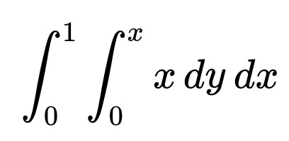
In words, for each x between 0 and 1, we take y from 0 up to x. Inside this region, the integrand is simply x. Evaluating:

The inner integral over y gives x multiplied by the length of the interval in y, which is x. Hence the inner integral becomes x · (x - 0) = x^2.

Then we integrate x^2 from x=0 to x=1, yielding 1/3.

Therefore the unconditional integral of x over x>y is 1/3. Dividing by the probability that x>y (which is 1/2) gives

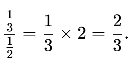
Hence E[X | X > Y] = 2/3.

Simulation Example in Python

Below is a quick simulation that can verify this result. We generate a large number of samples from Uniform(0,1) for both X and Y, and we then approximate E[X | X > Y] empirically.

import numpy as np

N = 10_000_000
X = np.random.rand(N)
Y = np.random.rand(N)

mask = (X > Y)
conditional_mean_estimate = X[mask].mean()
print(conditional_mean_estimate)

When run, conditional_mean_estimate will be close to 0.666..., illustrating the analytical result of 2/3.

Solution Summary

Because X and Y are i.i.d. Uniform(0,1), the probability that X > Y is 1/2. Within the region x > y in the unit square, the average value of X evaluates to 1/3 as an integral. Dividing 1/3 by 1/2 gives the final answer of 2/3.

What if we wanted E[Y | X > Y]?

By symmetry, one could argue that E[Y | X > Y] must be 1 - E[X | Y > X] if you do a direct approach, or more simply recognize that due to symmetry E[X | X > Y] + E[Y | Y > X] must sum to 1, but each event is the same measure. In fact, one can perform an identical integral just replacing roles of X and Y to get 1/3 for E[Y | X > Y]. This is because on the set X > Y, we are looking at the lower part of the square for Y, whose average ends up being 1/3.

How do we handle a different distribution for X and Y?

If X and Y have some other distribution, not necessarily uniform, the answer can change significantly. The probability P(X > Y) will be computed from their joint distribution, and the expression for E[X | X > Y] involves an integral of x over that region divided by the probability. Concretely, for continuous X and Y with PDFs f_X(x) and f_Y(y), we would need to evaluate something along these lines:

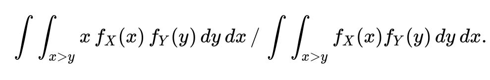
This can become more complex if X and Y are not independent or not uniformly distributed, and you would need the correct joint PDF to solve the integral.

Why is P(X > Y) = 1/2 when X and Y are i.i.d. Uniform(0,1)?

We can see this from the geometry of the unit square, which is of area 1. The region X > Y is the half of the square above the diagonal, which has area 1/2. Formally, for any continuous distribution that is symmetric and identical for X and Y, P(X > Y) = 1/2 because of that symmetry (assuming there is zero probability that X = Y in the continuous case, which is indeed 0 for the uniform distribution).

Could we have solved it purely by symmetry?

Yes, there is a way to argue purely by symmetry. One approach is to note that (X, Y) in the unit square is uniformly distributed, so the diagonal partitions the square into two equal areas. Then note that if we consider the average of X in the triangular region X > Y, we expect it to be located “farther” along the x-axis than in the entire square, suggesting the result 2/3. But the integral-based method is the most standard approach for a rigorous proof.

What if we think about an alternative direct approach?

One alternative approach might be: Condition on the fact that X > Y. Let Y = y, then X must be in (y, 1). You can integrate over y in (0,1) and the conditional PDF is normalized accordingly. This approach leads to the same integral result. It is simply another viewpoint on the same derivation.

Are there any traps or pitfalls an interviewee might fall into?

One common pitfall is to assume that E[X | X > Y] equals 0.5 because they might guess the midpoint of (0,1). That is incorrect because, given that X exceeds Y, X skews toward the higher side of the (0,1) interval. Another trap is to forget to divide by the probability that X > Y. An interviewee might just compute the integral of x in the region x > y to get 1/3, but then forget that we must normalize by P(X > Y) = 1/2, leading to the 2/3 final result.

How might this concept generalize to higher dimensions or transformations?

You can imagine if X and Y were vectors or from other distributions, you would look for the volume in n-dimensional space where certain constraints hold, compute the integral of X, and then normalize by the probability of that constraint. It is a straightforward generalization once you see how to handle integrals over constrained domains, but the simplicity of the uniform (0,1) distribution is what makes this particular problem neat.

Final answer to the original question

E[X | X > Y] = 2/3.

Below are additional follow-up questions

What if we define a new random variable Z = min(X, Y) and want E[Z | X > Y]?

When we consider the random variable Z = min(X, Y), on the event X > Y we know that Y < X, so Y = min(X, Y) in that situation. Therefore, within the region where X > Y, we have Z = Y. Hence we are effectively asked: “What is the expected value of Y given X > Y?”

To find E[Z | X > Y], we can exploit the fact that Z = Y in the region of interest. This then boils down to finding E[Y | X > Y].

By symmetry between X and Y in their joint uniform (0,1) distribution, we already know from direct integrals (or from reasoning about the geometry of the unit square) that E[Y | X > Y] = 1/3. Hence:

E[min(X, Y) | X > Y] = 1/3.

A potential subtlety here is to confirm that within X > Y, we don’t have a new “distribution” for Y that changes its overall shape drastically. Indeed, Y remains uniformly distributed but only in the subset of the plane where y < x. Intuitively, it “skews” to smaller values, making the expected value 1/3 rather than the unconditional mean of 1/2.

A practical pitfall would be forgetting that “min(X, Y)” becomes “Y” specifically on the event X > Y, so you might accidentally conflate it with the unconditional distribution of Y or do extraneous integrals. Another subtlety is ensuring you include the correct normalization factor (the probability that X > Y) if you try to compute from first principles.

How would the situation change if X and Y are independent but each have a different uniform range, say X ∼ Uniform(a, b) and Y ∼ Uniform(c, d)?

When X and Y do not share the same interval, the probability that X > Y and the conditional expectation E[X | X > Y] can shift significantly. For X ∼ Uniform(a, b) and Y ∼ Uniform(c, d):

1. The probability P(X > Y) involves the area in the (x, y) plane where x > y, restricted to a ≤ x ≤ b and c ≤ y ≤ d. You’d need to integrate over that rectangle’s intersection with x > y.

2. The conditional expectation E[X | X > Y] is computed by

( \frac{\int \int_{x>y, x \in [a,b], y \in [c,d]} x , dx , dy}{P(X > Y)}. )

Depending on how [a, b] and [c, d] overlap, you might get different geometric regions. If [a, b] and [c, d] do not overlap at all (e.g., b < c), then P(X > Y] might be 0 if the entire support of X is below the support of Y, or 1 if the entire support of X is above the support of Y. That is a tricky edge case:

• If b < c, then we always have x < y, so P(X > Y) = 0, making E[X | X > Y] undefined. • If a > d, then x > y always, so P(X > Y) = 1, and E[X | X > Y] = E[X] = (a + b)/2 in that degenerate scenario.

In more typical partially overlapping intervals, you’d have to carefully partition the integral region into slices where the intervals overlap or do it purely geometrically.

A major pitfall is to assume that the result 2/3 from the standard (0,1) uniform scenario applies regardless of the intervals. Another common mistake is failing to correctly handle partial overlaps where only part of [a, b] intersects [c, d], in which case the region x > y is truncated in a more complicated manner.

How would E[X | X > Y] differ if X and Y are no longer independent but still Uniform(0,1) marginally?

If X and Y have a correlation or dependence structure (while each marginally remains Uniform(0,1)), the probability that X > Y can deviate from 1/2, and the conditional distribution of X given X > Y might also shift.

Consider a case where X and Y are positively correlated. Intuitively, if Y is large, X also tends to be large. This might increase the probability that X > Y above 1/2, or it might shift E[X | X > Y] in ways that are not obvious without the exact form of the joint distribution. One must compute:

( P(X > Y) = \int \int_{x>y} f_{X,Y}(x, y) , dx , dy, )

and

( E[X | X > Y] = \frac{\int \int_{x>y} x , f_{X,Y}(x, y) , dx , dy}{P(X > Y)}. )

A subtlety with correlation is that the shape of f_{X,Y}(x,y) may favor or penalize certain regions. If X and Y follow, for instance, a Gaussian copula that forces them to be correlated, the region near the diagonal might hold different masses. The entire approach requires knowledge of the joint PDF.

A potential pitfall is to assume independence-based reasoning or geometry from the uniform square still holds. Another subtlety is ensuring that you handle the conditional PDF correctly if you try to compute E[X | X > Y] directly from f_{X,Y}(x,y)/(P(X > Y)).

What happens if we define a discrete analogue, where X and Y are discrete random variables uniformly distributed on {1, 2, ..., n}? How would we compute E[X | X > Y] in that context?

When X and Y are discrete uniform on {1, 2, ..., n} and independent:

• P(X = x) = 1/n for x ∈ {1, 2, ..., n}, and similarly for Y. • P(X > Y) = sum over x>y of P(X = x, Y = y) = 1/n² times the count of pairs (x, y) with x>y. That count is n(n−1)/2. So P(X > Y) = (n(n−1)/2) / n² = (n−1)/(2n).

Then,

( E[X | X > Y] = \frac{\sum_{x=1}^n \sum_{y=1}^{x-1} x \times \frac{1}{n^2}}{(n-1)/(2n)}. )

We sum x for all y < x (so from y=1 to y=x−1). This sum is ( \sum_{x=2}^n \left( x \times (x-1) \right) ) because for each x, there are (x−1) possible y values. Factoring out 1/n² from the probability, we get

( \sum_{x=2}^n x(x-1) = \sum_{x=2}^n (x^2 - x). )

We can use formulae for sums of squares and sums of integers:

( \sum_{x=1}^n x^2 = \frac{n(n+1)(2n+1)}{6}, \quad \sum_{x=1}^n x = \frac{n(n+1)}{2}. )

So

( \sum_{x=2}^n (x^2 - x) = \left(\sum_{x=1}^n x^2\right) - 1^2 - \left(\sum_{x=1}^n x\right) + 1. )

Evaluating those sums carefully gives a closed-form expression. Then we divide by n² for the probability factor and finally divide by (n−1)/(2n).

A subtlety is that as n → ∞, we might expect the discrete uniform distribution to approximate the continuous (0,1) scenario. Indeed, in the limit of large n, E[X | X>Y] / n should converge to 2/3.

Pitfalls: incorrectly counting the number of (x, y) pairs that satisfy x>y or mixing up the summation indices can yield a wrong formula. Another pitfall is forgetting that the probability for each pair is 1/n². Yet another subtlety is the boundary conditions x=1 or y=1, especially in partial sums.

How can we generalize E[X | X > Y] to other functions, for example E[f(X) | X > Y]?

Sometimes an interviewer may probe your ability to handle a more complex function. Instead of wanting E[X | X > Y], they might want E[f(X) | X > Y] for some function f, e.g., f(X) = X² or f(X) = exp(X).

The general approach is:

( E[f(X) \mid X > Y] = \frac{\int \int_{x>y} f(x) , f_X(x) f_Y(y) , dx , dy}{P(X > Y)}. )

If X and Y remain i.i.d. Uniform(0,1), we can attempt to write this as

( \frac{\int_0^1 \int_0^x f(x) , dy , dx}{1/2} = \frac{\int_0^1 f(x) , (x - 0) , dx}{1/2} = 2 \int_0^1 x , f(x) , dx, )

because the probability P(X > Y) is 1/2, and in the region 0 ≤ y ≤ x ≤ 1, we have y from 0 to x. Then we interpret that integral for the specific function f. For instance:

• If f(x) = x, we get 2 ∫₀¹ x · x dx = 2 ∫₀¹ x² dx = 2 × (1/3) = 2/3, which is the classic result. • If f(x) = x², we get 2 ∫₀¹ x · x² dx = 2 ∫₀¹ x³ dx = 2 × (1/4) = 1/2.

A subtlety is to ensure you multiply by x in the inner integral if you’re directly setting up the double integral carefully. Another potential pitfall is mixing up the difference between E[f(X) | X > Y] and E[X | X > Y] if you try to do a direct formula without carefully checking the integrand.

What if an interviewer asks about an application scenario, such as gambler’s ruin or betting strategies, relating to the concept of E[X | X > Y]?

One real-world question might be: “If two players each pick a random number from (0,1), and you must guess who will have the higher number, what is the expected value of the higher number? And how does E[X | X>Y] come into play in designing a strategy?”

A direct answer is that if you guess the higher number after seeing them, you trivially guess correctly. But if you have to guess “X or Y” before seeing them, the probability that X is the higher number is 1/2, and the expected higher number overall is 2/3. However, one might also be asked: “Given that we learned X > Y, how might that knowledge help in a game scenario?” Well, if you discover X is indeed greater, you know X is on average 2/3. But that by itself might not guarantee a winning strategy unless you also have some cost function or comparison to Y’s value.

A subtlety is that if the game has payoffs that depend on the difference (X - Y), you might need E[X - Y | X > Y]. That can be computed similarly by taking the integral of (x - y) over the region x>y, then dividing by P(x>y). This gives 1/6 for E[X - Y | X > Y], because the integral of (x - y) in that region is 1/6, and normalizing by 1/2 yields 1/3 if you consider the entire region. Actually, you’d do:

( \int_0^1 \int_0^x (x - y) , dy , dx = \int_0^1 \left[x \cdot (x) - \frac{x^2}{2}\right] dx = \int_0^1 \left[x^2 - \frac{x^2}{2}\right] dx = \int_0^1 \frac{x^2}{2} dx = \frac{1}{6}. )

Then dividing by 1/2 yields 1/3.

Pitfalls: mixing up the unconditional difference E[X - Y] with the conditional difference E[X - Y | X > Y]. Another subtlety is ensuring that you set up integrals correctly or interpret probability statements carefully in game or betting contexts.

Suppose the event is X > Y + a certain threshold δ > 0. How would we compute E[X | X > Y + δ] in the uniform (0,1) scenario?

Now the condition is stricter: X must exceed Y by at least δ, where δ is in (0,1). We can set up:

( P(X > Y + \delta) = \int_0^1 \int_0^1 \mathbf{1}(x > y + \delta) , dx , dy )

in the unit square. Geometrically, that’s the region above the line x = y + δ, which is a band that starts δ units above the diagonal y=x-δ. The feasible range for y is 0 ≤ y ≤ 1−δ, and for each y, x must lie in (y+δ, 1).

Hence:

( P(X > Y + \delta) = \int_0^{1-\delta} \int_{y+\delta}^1 dx , dy = \int_0^{1-\delta} [1 - (y+\delta)] , dy = \int_0^{1-\delta} (1 - y - \delta) , dy. )

Evaluating that integral:

( = \int_0^{1-\delta} 1 , dy - \int_0^{1-\delta} y , dy - \int_0^{1-\delta} \delta , dy = (1-\delta) - \frac{(1-\delta)^2}{2} - \delta (1-\delta). )

We can simplify that, but it’s typically easier to keep it in a piecewise manner or do a direct symbolic manipulation. Then we compute:

( E[X | X > Y + \delta] = \frac{\int_{y=0}^{1-\delta} \int_{x=y+\delta}^1 x , dx , dy}{P(X > Y + \delta)}. )

In each slice y is from 0 to 1−δ, and x is from y+δ to 1, so the inner integral of x dx from x=y+δ to x=1 is:

( \left[\frac{x^2}{2}\right]_{y+\delta}^1 = \frac{1}{2} - \frac{(y+\delta)^2}{2}. )

Summing that over y from 0 to 1−δ yields:

( \int_0^{1-\delta} \left(\frac{1}{2} - \frac{(y+\delta)^2}{2}\right) dy. )

This can be evaluated exactly. Dividing that result by P(X > Y + \delta) will give E[X | X > Y + \delta].

Pitfalls: forgetting to shift the region properly by δ, or incorrectly letting y exceed 1−δ, or ignoring the condition that for y close to 1, x might not be able to exceed y + δ. Another subtlety is whether δ is small or large: if δ > 1, then P(X > Y + δ) = 0, which is a degenerate case.

What if we make a transformation from the X-Y plane to new variables, such as U = X + Y and V = X - Y?

A sophisticated interviewer might ask: “Can you solve for E[X | X>Y] by converting to a new coordinate system, say U = X+Y and V = X−Y?”

• In that transformation, X = (U+V)/2 and Y = (U−V)/2. • The event X>Y implies V>0. • For uniform (0,1) i.i.d., the region 0 < x < 1, 0 < y < 1 translates to constraints on U and V: 0 < (U+V)/2 < 1 and 0 < (U−V)/2 < 1.

Those constraints become 0 < U+V < 2 and 0 < U−V < 2, which rearranges to −U < V < U and U−2 < V < 2−U. So the domain is the intersection of: V < U, V > −U, V < 2−U, V > U−2.

Inside that domain, V>0 defines a subregion. Once you find that subregion, you might integrate (U+V)/2 times the joint PDF in (U, V) space. The Jacobian of the transformation from (X,Y) to (U,V) is 1/2 in absolute value.

A subtlety is that dealing with piecewise constraints can become quite elaborate in the unit square, so you must carefully map each corner. A major pitfall is incorrectly translating the region 0<x<1, 0<y<1 into the (U,V) domain and forgetting the factor from the Jacobian.

Nevertheless, the result, once integrated, will match 2/3 for E[X | X>Y]. But an interviewer might simply be checking your comfort with changes of variables for double integrals, so you should be able to articulate the steps.

Suppose we are asked to verify E[X | X>Y] = 2/3 with a small number of Monte Carlo samples, and our estimate is off. What might cause an incorrect simulation result?

Common pitfalls in simulations:

• Seeding your random generator incorrectly or not seeding at all, leading to different results in small-sample runs. • Using a small N, e.g., 100 or 1,000, might cause higher variance and you might not get an estimate near 2/3. • Confusion about the event X>Y: maybe you wrote code that checks X≥Y or y>x by accident. Any off-by-one or sign bug will produce the wrong subset for the average. • Overflow or underflow issues are less likely in typical Uniform(0,1) simulations, but with extremely large arrays or unusual library calls, you might break typical assumptions. • Failing to handle the case that Y might be equal to X. Even though that has measure zero in continuous sampling, in numerical simulations with limited floating-point precision, you could have ties that you accidentally treat as “greater than.”

To mitigate these issues, you’d confirm your condition check, do repeated runs with larger N to reduce variance, and compare your final sample-based estimate to the expected 2/3 value.

How would you estimate E[X | X>Y] if X, Y ~ Uniform(0,1) are not known a priori, but you have empirical samples from some real-world process?

In practice, you might have data where you collect i.i.d. pairs (x_i, y_i) that you believe come from some distribution, possibly near uniform but not guaranteed. To approximate E[X | X>Y], you can:

1. Filter the dataset to only those points where x_i > y_i.

2. Compute the sample average of x_i in that filtered set.

This empirical average approximates E[X | X>Y]. If the distribution truly is uniform (0,1), the result should converge near 2/3 as the sample size grows. But if the real data deviate from uniform, the estimate may differ.

Edge cases or pitfalls include:

• You might discover that your real data do not uniformly populate the region (0,1). In that case, the result might be systematically higher or lower than 2/3. • If the number of data points is too small or if the subset where X>Y is small (imagine a case where X>Y is rare due to the data collection process), you might get a high-variance estimate.

Additionally, if X and Y are correlated in real data, your assumption of independence or uniform distribution is violated, and the theoretical 2/3 no longer applies.

If we suspect X and Y have outliers or a heavy-tailed distribution, how does that affect a real-world computation of E[X | X>Y]?

For heavy-tailed distributions, it’s possible that extreme values of X or Y will dominate the region X>Y. For instance, if X and Y follow some Pareto distribution, the probability that X>Y might be quite different from 1/2, and E[X | X>Y] could be dominated by the tail behavior of X.

This means that a small fraction of observations with very large X could significantly inflate the average. If you do an integral approach, you must carefully handle the infinite or semi-infinite domain. If you do a simulation, you must ensure you have enough samples to capture tail events.

A key pitfall is that naive sampling might severely underestimate tail events unless your sample is very large, causing an underestimate or overestimate of E[X | X>Y]. Another subtlety is that if Y also can become extremely large, the condition X>Y might systematically exclude certain tail events. It really depends on the distribution specifics, so you have to do the full integral or a careful simulation-based approach that accommodates heavy tails.

Could we interpret E[X | X>Y] in terms of rank statistics or order statistics?

One interesting perspective is that if X and Y are i.i.d. continuous random variables, then (X, Y) is effectively a sample of size 2 from that distribution. The condition X>Y means we’re looking at the maximum in some sense. Actually, we are focusing on the random variable that ended up on top in that pair.

If we had X₁, X₂, ..., Xₙ i.i.d. Uniform(0,1), we know the expected maximum of all n samples is n/(n+1). For n=2, that maximum is 2/3. But note that the maximum of two samples is exactly the random variable among X and Y that ended up larger. Indeed, E[max(X, Y)] = 2/3 for i.i.d. Uniform(0,1). This is exactly E[X | X>Y] if we label the larger sample “X.”

A potential confusion or subtlety is that the random variable we label “X” from the start might not always be the max if we consider them unlabeled. But if from the beginning we fix the identity as “X” and “Y,” then E[X | X>Y] matches the expected value of the winner’s sample in a random 2-sample draw from Uniform(0,1).

Pitfalls: mixing up the naming convention or not realizing that E[X | X>Y] is the same as E[max(X,Y)] when X and Y are labeled i.i.d. Another subtlety is that if X and Y had different distributions or a correlation, that equivalence to a rank statistic interpretation breaks down.

How might these results change if the domain for X and Y is not (0,1) but some bounded region [0,1]×[0,1] with additional constraints like X + Y ≤ 1?

If we had the constraint X + Y ≤ 1, for instance, we might be dealing with random variables distributed uniformly in the triangular region of the square bounded by x + y ≤ 1. That region is half the unit square but oriented differently from the x>y diagonal. Then the event X>Y intersects that triangular region in a smaller subregion.

We would need to carefully compute:

• P(X>Y and X + Y ≤ 1). • Then E[X | X>Y, X + Y ≤ 1], or E[X | X>Y], but with the new domain.

The integration becomes a geometry problem. We might end up with a region shaped by lines x>y and x+y≤1, which is a wedge in the unit square. Integrating x over that wedge and dividing by the measure of the wedge yields the conditional expectation.

A subtlety is that we have to be absolutely certain about how the uniform distribution is defined. Is it uniform on the entire square and then we only consider points that also satisfy x+y≤1, or is it uniform only on the triangle x+y≤1? These are different distributions. A pitfall is to assume the same area-based approach from the entire square (0,1)×(0,1) still applies unaltered. Another subtlety is normalizing by the appropriate probability measure in that truncated domain.

What if the interview follows up with a question about the role of conditional expectation in regression tasks or deep learning models?

Although the question about E[X | X>Y] might seem purely mathematical, an interviewer could pivot to how this concept arises in machine learning:

• Conditional expectation under constraints can be related to partial dependence or conditional distributions in regression. For example, you might have a model that outputs X (some performance metric) conditioned on some event Y (some threshold being exceeded). • In a deep learning context, you could imagine training a neural network that predicts the conditional mean of X given an event. The network’s loss could be MSE on data for which X>Y.

Potential pitfalls: applying the law of large numbers incorrectly when you only have data for certain events. Also, if Y is itself predicted by another model, you have correlation or nested dependencies to consider.

A subtlety is that in real ML tasks, X and Y might be features with complicated distributions, so the beautiful uniform solution is no longer valid. Another subtlety is that partial data segmentation (like X>Y) might lead to biased training sets or concept drift if Y is not stable.

Are there any real-world engineering examples where E[X | X>Y] specifically is needed?

An interviewer might test your ability to connect the concept to practical scenarios:

• Reliability analysis: Suppose X is the time to failure of component A, and Y is the time to failure of component B, each distributed uniformly over some time range (though real-world times to failure are rarely uniform, but consider a simplified scenario). If you condition on A failing after B (i.e., X>Y), you might want the expected time of A’s failure in that scenario for planning or cost analysis. • Auction or bidding scenarios: If you place a random bid X and your competitor places a random bid Y, you might want E[X | X>Y], to see what your expected bid is when you outbid the competitor. This might tie into game theoretic strategies or second-price auctions.

Pitfalls in engineering contexts include ignoring the real distribution of times to failure or bids. Another subtlety is that uniform might be a severe oversimplification, so you must adapt the integral-based method to the actual distribution or collect data to estimate it.

What if we interpret E[X | X>Y] as a measure of “dominance” in repeated games and consider advanced topics like the probability that X is an ϵϵ-dominant strategy?

An interviewer might probe your knowledge of advanced probability and game theory:

1. We define an ϵϵ-dominant region as X>Y+ε for some small ε>0. Then we compute P(X>Y+ε) or E[X | X>Y+ε].

2. This can be extended to think about how often one strategy (X) outperforms another (Y) by a margin of at least ε, and what the expected performance is in that scenario.

A subtlety is that in repeated random draws from X and Y, we might see that the fraction of times X is bigger than Y by at least ε is not simply P(X>Y+ε) if X and Y are correlated or not identically distributed. Another pitfall is that if the domain is unbounded, the integrals might not converge, or might require careful tail analysis.

Overall, one must revert to the fundamental approach: define the event in question, compute its probability, integrate the function of interest over the region that satisfies the event, and then normalize by that probability.