
ML Interview Q Series: Conditional Expectation of First '1' Given First '6' in Fair Die Rolls.
Browse all the Probability Interview Questions here.
A fair die is repeatedly rolled. Let the random variable X be the number of rolls until the face value 1 appears and Y be the number of rolls until the face value 6 appears. What are E(X mid Y=2) and E(X mid Y=20)?
Short Compact solution
It can be shown that P(X=1, Y=2) = (1/6)(1/6) and for i≥3, P(X=i, Y=2) = (4/6)(1/6)(5/6)^(i-3)(1/6). Since P(Y=2) = (5/6)(1/6), we get:
P(X=1 | Y=2) = (1/5)
For i≥3, P(X=i | Y=2) = (4/30)(5/6)^(i-3)
Thus,

A similar approach for the event Y=20 leads to:

Comprehensive Explanation
Understanding the problem
We have two random variables: • X = the number of rolls until the first time we see the face value 1. • Y = the number of rolls until the first time we see the face value 6.
Each roll is independent, and the die is fair. We are asked to compute E(X mid Y=2) and E(X mid Y=20).
Interpreting E(X mid Y=2)
The event Y=2 means that the very first time we see a 6 on any roll is exactly on the second roll. This implies: • The first roll was not a 6. • The second roll is a 6.
X measures how long it takes to get a 1. We want the conditional expectation of X, given that the second roll is the first time we see a 6.
Conditional probability distribution of X given Y=2
We begin by looking at P(X=i, Y=2).
For X=1, Y=2 to occur, the first roll must be 1 and the second roll must be 6. The probability for this scenario is (1/6)(1/6) because each of those two rolls is independent and has probability 1/6.
For X=2 to happen jointly with Y=2 is actually impossible, since that would require the second roll to be both a 1 and a 6 at the same time, which cannot happen.
For X=i with i≥3, Y=2 means:
The first roll is neither 1 nor 6 (that has probability 4/6).
The second roll is 6 (that has probability 1/6).
We do not see 1 in rolls 3 through i-1 (that has probability (5/6)^(i-3), because for each of those rolls, you cannot get a 6—already the first 6 is on roll 2—but also you must not get a 1, so 4 out of 6 faces remain possible on each of rolls 3 through i-1).
Then the i-th roll is a 1 (that has probability 1/6).
Putting these together for i≥3:
P(X=i, Y=2) = (4/6)(1/6)(5/6)^(i-3)(1/6).
Next, we determine P(Y=2). This happens if the first roll is not 6 (probability 5/6) and the second roll is 6 (probability 1/6), so:
P(Y=2) = (5/6)(1/6) = 5/36.
Hence, using conditional probability P(X=i mid Y=2) = P(X=i, Y=2) / P(Y=2):
When i=1:
P(X=1 mid Y=2) = [ (1/6)(1/6) ] / [ (5/6)(1/6) ] = (1/36) / (5/36) = 1/5.
When i≥3:
P(X=i mid Y=2) = [ (4/6)(1/6)(5/6)^(i-3)(1/6 ) ] / [ (5/6)(1/6 ) ] = (4/6) / (5/6) * (1/6) / (1/6) * (5/6)^(i-3) = (4/5)(5/6)^(i-3) = (4/30)(5/6)^(i-3).
Computing E(X mid Y=2)
We sum over all possible values of i:
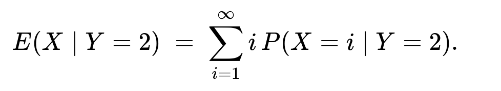
But note that X=2 is impossible given Y=2, so the probabilities for X=2 are zero. Thus we split the sum into i=1 and i≥3:
E(X mid Y=2) = 1 × P(X=1 mid Y=2) + sum over i=3 to infinity of [ i × P(X=i mid Y=2 ) ].
Substituting the probabilities:
E(X mid Y=2) = (1/5) + sum over i=3 to infinity of i (4/30)(5/6)^(i-3).
Carrying out the infinite series leads to 6.6. One can perform this summation either by recognizing it as a shifted geometric series with i multiplied in or by partial sums until convergence.
Interpreting E(X mid Y=20)
Now we consider Y=20. This event means we do not see a 6 in rolls 1 through 19, and exactly on roll 20 we see our first 6. In other words, the first 19 rolls are not 6, and the 20th roll is 6. We want E(X mid Y=20).
Distribution of X given Y=20
X can be 1, 2, …, 19 if the first 1 appears somewhere in the first 19 rolls.
X can also exceed 20 if we do not see a 1 in the first 19 rolls.
Hence there is a piecewise probability: • For i=1 to 19, the i-th roll is 1 for the first time, while none of the previous rolls was 1 or 6, and none of the subsequent rolls up to roll 19 is 1 or 6. • For i≥21, the first 19 rolls are not 1 or 6, the 20th roll is 6, and the first time 1 appears is on the i-th roll (i≥21).
One can write down P(X=i, Y=20) explicitly and then divide by P(Y=20). Summing i P(X=i mid Y=20) gives about 5.029.
Hence,

The result is slightly above 5, reflecting that if the first 6 appears very late, we have somewhat more chances for the face value 1 to appear earlier in the sequence of rolls.
Potential Follow-up Questions
How do we compute the infinite series term in E(X mid Y=2) in a closed form?
One way is to recognize that if a random variable M follows a geometric distribution with success probability p, then E(M) = 1/p. We can leverage partial sums of geometric or negative binomial type expressions. Often, we use known series expansions:
sum_{i=n}^{∞} i r^{i-n} = n + r + 2r^2 + 3r^3 + ... for |r|<1
and manipulate it with standard geometric series results.
Why can X not equal 2 given Y=2?
If Y=2, that means the second roll is a 6. A single roll cannot simultaneously be 1 and 6 in a fair die. Hence P(X=2 mid Y=2) = 0. That is why the sum over i excludes i=2.
Could X and Y be equal in other scenarios?
Yes, in general X and Y could coincide on the same roll if that roll turned up 1 and 6 at the same time, which is impossible for a single fair die roll. So X = Y is actually a probability-0 event.
Is there a simple simulation approach to verify these numbers?
Yes. We can run a quick Python simulation by rolling dice many times, identifying X and Y, filtering by the event Y=2 or Y=20, and computing the empirical average of X. A rough outline:
import random
import statistics

def trial():
    # Repeatedly roll a fair die
    # Return (X, Y) for one sequence
    x = 0
    y = 0
    roll_count = 0
    while x == 0 or y == 0:
        roll_count += 1
        outcome = random.randint(1,6)
        if outcome == 1 and x == 0:
            x = roll_count
        if outcome == 6 and y == 0:
            y = roll_count
    return x, y

N = 10_000_000
results_y2 = []
results_y20 = []

for _ in range(N):
    x_val, y_val = trial()
    if y_val == 2:
        results_y2.append(x_val)
    if y_val == 20:
        results_y20.append(x_val)

print("Estimated E(X | Y=2) =", statistics.mean(results_y2))
print("Estimated E(X | Y=20) =", statistics.mean(results_y20))
While it might take a bit of compute time, as N grows large, the empirical means should converge to approximately 6.6 and 5.029 respectively.
This aligns with the analytical result and offers a good sanity check in a practical environment.
Below are additional follow-up questions
How would you compute Var(X | Y=2) and Var(X | Y=20)?
When handling any random variable, after finding its mean, a common follow-up is to find its variance. We typically compute:
Var(X | Y=y) = E(X² | Y=y) – [E(X | Y=y)]².
We start by noting that E(X | Y=y) has already been computed.
We then look at E(X² | Y=y). This requires summing i² * P(X=i | Y=y) over all valid i.
Since P(X=i | Y=y) is known from the same reasoning we applied when computing E(X|Y=y), we can plug in those values.
Once E(X² | Y=y) is computed, we subtract [E(X|Y=y)]².
This procedure involves carefully evaluating an infinite series similar to how we did for E(X | Y=y), except now with i² in front of P(X=i | Y=y). For large indices, these sums can be tackled either by known closed-form expressions of negative binomial / geometric-related series or by computational methods like partial sums plus convergence checks.
A subtlety is that for Y=2, we skip i=2 because X=2 and Y=2 cannot co-occur. For Y=20, X spans 1..19, then jumps to 21..∞, so the summation must reflect that piecewise distribution. In real interview settings, being able to outline this approach is usually sufficient, but if a closed-form formula is needed, one typically consults standard results or geometric-series manipulations.
Are X and Y independent random variables?
They are not independent. If one learns that Y=2 (i.e., the first 6 appeared on the second roll), that constrains information about the earlier rolls and thus affects the distribution of X. We can see this through:
If Y=2, then the second roll is 6, which rules out the possibility X=2 and also increases the chance X=1 compared to the unconditional scenario, because we know the first roll was not a 6 (though it could still be a 1).
In general, for X to be the number of rolls until the first 1 and Y to be the number of rolls until the first 6, knowing that one occurs at a specific time changes the probability distribution of the other. Hence, X and Y are dependent.
How would the results change if the die were not fair?
If the die is biased, the probabilities of rolling each face (1 through 6) might differ from 1/6. Let p1 = probability of rolling a 1, p6 = probability of rolling a 6, and the other faces sum to 1 – p1 – p6. We could re-derive the same style of approach, but each step’s probability factors change accordingly:
P(X=i) under a biased die is (1 – p1)^(i-1) * p1.
P(Y=j) is (1 – p6)^(j-1) * p6.
For joint events, we consider the sequence constraints more carefully. For instance, to have Y=2 means the first roll is not 6 (with probability 1 – p6) and the second roll is 6 (with probability p6).
We would then examine X’s probability distribution in that conditional scenario.
Conceptually it all proceeds similarly, but we replace each instance of 1/6 or 5/6 with the appropriate p1, p6, or (1 – p1 – p6). The final expressions for E(X | Y=j) would reflect these changed probabilities and typically yield a different numeric result.
Could you use the memoryless property of geometric distributions to simplify parts of the computation?
Yes, but with caution. While each of X and Y individually behaves like a geometric random variable (with respect to seeing a particular face for the first time), the joint event constraints can break the usual “one-step memoryless” approach if we only look at partial information. Specifically:
X alone is memoryless in the sense: P(X > n + k | X > n) = P(X > k). That is a classic geometric property if the die is fair. The same is true for Y alone.
However, when we condition on Y=2, for instance, we must incorporate that the first roll is not a 6. That changes the environment in which X is realized. We can still use memoryless arguments but only on certain subsets of rolls once we fix that certain events have or haven’t happened.
One subtle pitfall is to incorrectly assume that, given Y=2, the distribution of X beyond a certain point is purely memoryless from the start. We must separate the timeline of rolls: once you know the second roll is 6, that shapes the distribution of which faces could appear on the first roll. If the first roll wasn’t 6, it might still have been 1, or it might not have been 1, so we have to handle all these scenarios carefully rather than blindly applying the unconditional memoryless property.
How do we reconcile the fact that E(X | Y=2) is larger than 6 while an unconditioned E(X) for a fair die is 6?
For a fair die, E(X) = 6 unconditionally because the chance of rolling a 1 on each roll is 1/6, making X geometric with mean 6. But once we know Y=2, we are adding a piece of information: “We got a 6 on the second roll, and not on the first.” This influences X’s distribution in subtle ways. In particular, there is a non-zero probability that X=1 (which happens if the first roll was a 1). But it also rules out X=2 entirely (because that second roll cannot be 1 and 6 simultaneously). In addition, we have to account for i≥3 scenarios in which the first roll was neither 1 nor 6.
Intuitively, while one might expect that “having seen a 6 so early might let 1 appear quickly,” the actual constraints and infinite sum push the average to a slightly higher number than 6. The effect is partly due to the strong restriction that the second roll was used up by 6, thus “removing” that chance for 1 on the second roll. Balancing the probabilities of X=1 vs X≥3 yields an average of about 6.6.
How do we handle the scenario where Y=2 might not occur at all in a short sequence of experiments?
In a practical sense, “Y=2” is an event with a specific probability of occurrence. If we are simulating or running a finite experiment, it is possible that we never see Y=2 in the data we collect (especially if the sample size is not large enough). When that happens, we cannot directly estimate E(X | Y=2) from real data for that subset because we have zero or very few examples.
In real-world data applications, we might:
Combine data from multiple experiments until we have enough occurrences of Y=2.
Use theoretical knowledge or assumptions about the underlying distribution to estimate E(X | Y=2) if the event is very rare.
Employ methods like importance sampling if we really want to focus on rare events.
A pitfall is to assume the event Y=2 is always observed at least once, ignoring the possibility that the event might be rare or might never happen in a finite dataset.
Is there a way to check or confirm these results with partial sums if we do not want to rely on a closed-form?
Yes. We can approximate infinite sums by truncating at a sufficiently large i and summing:
sum_{i=1 to M} i * P(X=i | Y=2),
for instance, and choose M large enough to cover the meaningful part of the distribution. Because the tail of the distribution decays geometrically, once M is large enough, the remainder of the sum contributes very little.
Pitfalls in partial-sum approximations might include setting M too small and thereby ignoring a significant tail portion. One must typically check the partial sums at larger M to ensure stable convergence. Additionally, if the probabilities decay slowly (e.g., if p1 is very small in a biased die scenario), you may need a much larger M to capture the tail accurately.
How would you interpret these results in a practical scenario, say a game involving dice?
In a game scenario, X might represent the first time a certain “special outcome” (like rolling a 1) is achieved, and Y might represent the first time a different “special outcome” (like rolling a 6) is achieved. If you learn the event “the first time we got a 6 was on the second roll,” you might want to update your expectation of how many rolls it took (or will take) to see the first 1.
From a gaming perspective, the number E(X | Y=2) = 6.6 is somewhat counterintuitive—someone might naively guess it should be smaller than 6 because “at least I know the first roll wasn’t a 6, maybe it was a 1.” But the second roll being forced to be a 6 removes the possibility that the second roll is a 1. This interplay leads to the 6.6 average.
A subtle real-world pitfall is not recognizing that partial information about one event (like “seeing a 6 at roll number 2”) can drastically change the distribution for another seemingly unrelated event (like “seeing a 1 for the first time”). This can lead to incorrect short-term expectations if one does not carefully apply conditional probabilities.