ML Interview Q Series: Conditional Probability for Three Distinct Dice Rolls Summing to 12 Using Combinatorics.

Browse all the Probability Interview Questions here.

7. Say you roll three dice and observe the sum of the three rolls. What is the probability that the sum of the outcomes is 12, given that the three rolls are different?

This problem was asked by Facebook.

A detailed way to approach this problem is to recognize that we are dealing with a conditional probability:

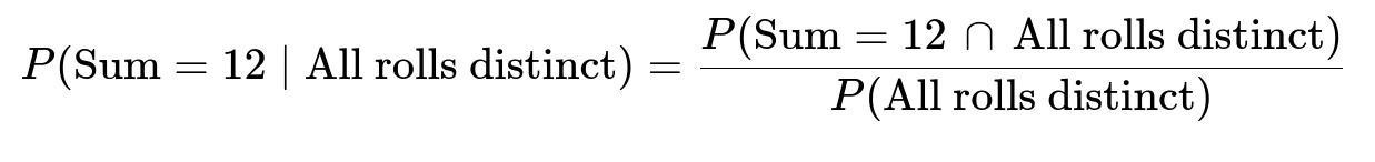
In plain language, we want to count how many total ways the dice can show three distinct values and, among those, how many ways yield a sum of 12.

Total number of possible outcomes (unconditional)

When rolling three fair six-sided dice (each die having faces {1, 2, 3, 4, 5, 6}), the total number of ways (ordered) to observe outcomes is:

• Each die can take 6 possible values.

• Therefore, total possible outcomes = 6 × 6 × 6 = 216.

Number of ways the three rolls are distinct

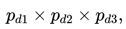
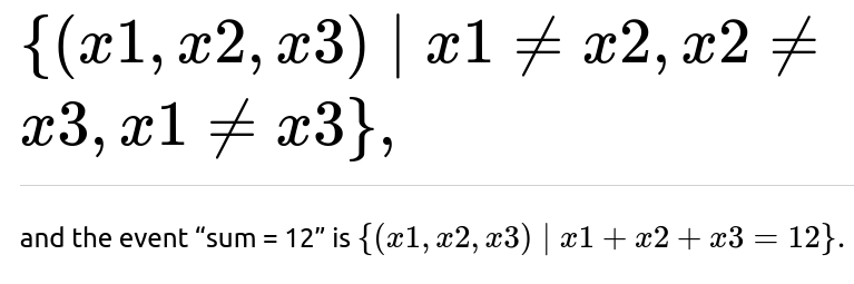
We want the count of ordered triples (d1, d2, d3) where d1, d2, d3 ∈ {1,…,6} and d1 ≠ d2, d2 ≠ d3, d1 ≠ d3. A standard approach is:

• Choose the value of the first die in 6 ways.

• The second die can be any of the remaining 5 distinct values.

• The third die can be any of the remaining 4 distinct values.

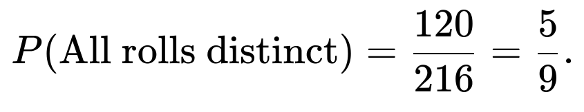
• Hence, the number of ways to have three distinct values = 6 × 5 × 4 = 120.

Thus:

Number of ways the sum is 12 with three distinct rolls

We now count how many ordered triples (d1, d2, d3) sum to 12 (i.e., d1 + d2 + d3 = 12) under the constraint that d1, d2, d3 are each in {1, …, 6} and distinct.

A systematic enumeration helps:

• The distinct combinations of three different dice faces summing to 12 are:

  • (1, 5, 6)

  • (2, 4, 6)

  • (3, 4, 5)

Check quickly that no other triplets meet both the distinctness and the sum to 12 requirement within 1 to 6. Each of the above sets has 3 distinct values, so each set of values can be permuted in 3! = 6 ways when we consider the dice as an ordered triple. Therefore:

• (1, 5, 6) gives 6 permutations.

• (2, 4, 6) gives 6 permutations.

• (3, 4, 5) gives 6 permutations.

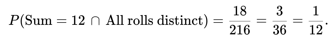
Total number of distinct-ordered triples summing to 12 = 6 + 6 + 6 = 18.

Hence:

Putting it all together

Substitute these counts into the conditional probability formula:

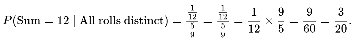
Therefore, the probability is 3/20, which is 0.15 (or 15%).

Why the probabilities and counts work out this way

The main reason behind these numbers is that once the dice have to show different values, it eliminates many possible repeats or duplicates in the outcomes, shrinking the total number of equally likely scenarios to 120 rather than 216. Among those, only a small subset (18 ways) reach a sum of 12 with each die showing a different face. The ratio of 18/120 then directly gives 3/20.

Subtleties and potential pitfalls

• It is easy to miscount the total “distinct” outcomes by forgetting that dice are considered ordered. For example, if someone were to use combinations (as though dice were unlabeled) without multiplying by permutations, that might lead to an incorrect total.

• Missing one of the valid (d1, d2, d3) triplets or counting an invalid one (such as values out of range or with duplicates) will yield an incorrect numerator.

• Another subtle point is the difference between enumerating combinations (e.g., {1,5,6}) versus permutations ((1,5,6), (5,1,6), etc.). Because each die is distinct in the real world (e.g., roll #1, roll #2, roll #3), we need to treat each ordered permutation as a separate outcome.

Python example to confirm the result

One way to cross-verify is simply to do a brute-force enumeration in Python:

count_all_distinct = 0
count_sum12_and_distinct = 0

for d1 in range(1, 7):
    for d2 in range(1, 7):
        for d3 in range(1, 7):
            if d1 != d2 and d2 != d3 and d1 != d3:
                count_all_distinct += 1
                if d1 + d2 + d3 == 12:
                    count_sum12_and_distinct += 1

prob_all_distinct = count_all_distinct / 216
prob_sum12_and_distinct = count_sum12_and_distinct / 216
conditional_prob = prob_sum12_and_distinct / prob_all_distinct

print("Number of distinct outcomes:", count_all_distinct)  # Should be 120
print("Number of ways sum=12 and distinct:", count_sum12_and_distinct)  # Should be 18
print("Conditional probability:", conditional_prob)  # Should be 3/20

Running this snippet would confirm:

• count_all_distinct = 120

• count_sum12_and_distinct = 18

• conditional_prob = 0.15 (i.e., 3/20)

Could you approach this using a generating function?

Yes, one can use a generating function technique, but it is often more complicated than a straightforward combinatorial count for this particular problem. The generating function for a single fair six-sided die is:

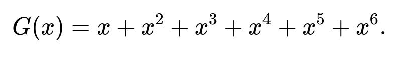
For three dice, the generating function is the cube of that polynomial:

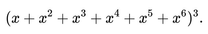
To incorporate the constraint that the three dice values must be distinct, one would have to exclude terms in which any power is counted multiple times for the same combination (i.e., an inclusion-exclusion approach to ensure each distinct die face is used at most once). Then you would look at the coefficient of ( x^{12} ) in the appropriately adjusted generating function. While it is possible, it is less direct than enumerating valid triples as we did.

Why are there exactly 120 ways for three dice to show distinct faces?

For ordered outcomes of three dice, each die can be viewed as a separate position in the triple (d1, d2, d3). If no two dice faces can be the same:

• The first die has 6 possible outcomes.

• The second die then has 5 possible outcomes (because it can’t match the first).

• The third die has 4 possible outcomes (because it can’t match the first or second).

Multiplying them yields 6 × 5 × 4 = 120. This matches well-known permutations logic: 6P3 = 6! / 3! = 6 × 5 × 4 = 120.

Are dice considered labeled or unlabeled in this problem?

They are considered labeled (or ordered) by default in typical probability settings unless otherwise stated. Each roll is a separate event, so rolling a 1, then a 5, then a 6 is distinct from rolling a 5, then a 1, then a 6. This distinction is critical to get the right count of total outcomes (216) and distinct outcomes (120).

If the dice were considered completely identical (unlabeled), then you would count combinations rather than permutations and use a different total set of outcomes. However, that is not the usual assumption when dealing with physical dice rolls.

Could there be a simpler direct enumeration for the sum of 12 and distinct faces?

Some people prefer to list all possible (d1, d2, d3) that sum to 12 and then filter for distinctness:

• All integer solutions to d1 + d2 + d3 = 12 with each d ∈ {1, …, 6}.

• Then remove any solutions that have repeated values.

That is essentially what we did by systematically identifying (1, 5, 6), (2, 4, 6), (3, 4, 5) as the only valid distinct sets of faces summing to 12. After that, one multiplies each unique set by 6 permutations.

What if someone forgot to multiply by 6 for each triplet?

They would wrongly count only 3 ways (for the sets {1,5,6}, {2,4,6}, {3,4,5}), leading them to compute 3 / 120 = 1/40 as the conditional probability. But that would neglect the fact that each set can appear in 6 possible permutations. This is a common mistake when switching between combinations (unlabeled sets) and permutations (ordered triples).

Are there real-world examples or edge cases to be mindful of?

In practical dice games, sometimes dice are truly indistinguishable physically. However, the usual assumption is that we track them as separate events: “the first roll is a 5, second is a 2, third is a 1.” Real-world pitfalls include:

• Mixing up labeled vs. unlabeled counting.

• Forgetting to account for or remove duplicates in the sum.

• Using partial enumerations or partial combinatorial arguments that omit or double-count some outcomes.

All of these can lead to small but crucial differences in final probability calculations.

Summary of the direct result

The probability that three fair, standard dice sum to 12 given that all three dice show different numbers is 3/20 (15%). This result is found by carefully counting the valid outcomes and dividing by the total number of distinct-outcome possibilities.

Below are additional follow-up questions

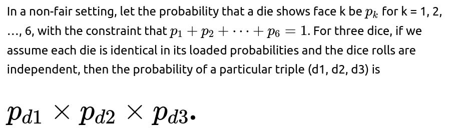
How would the approach change if the dice were not fair?

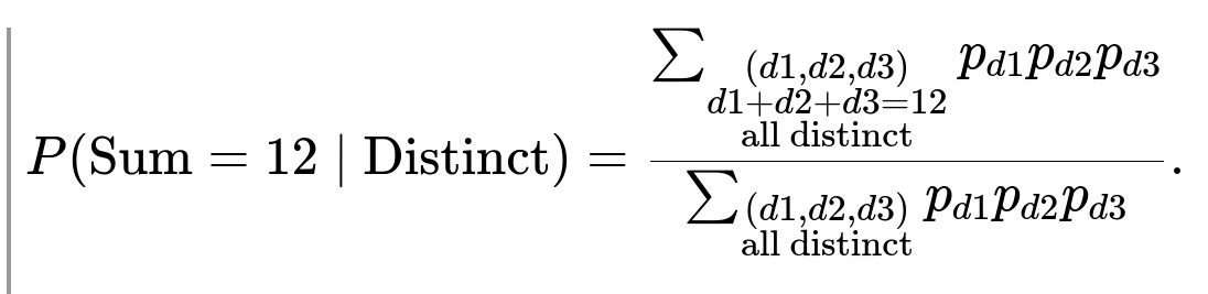
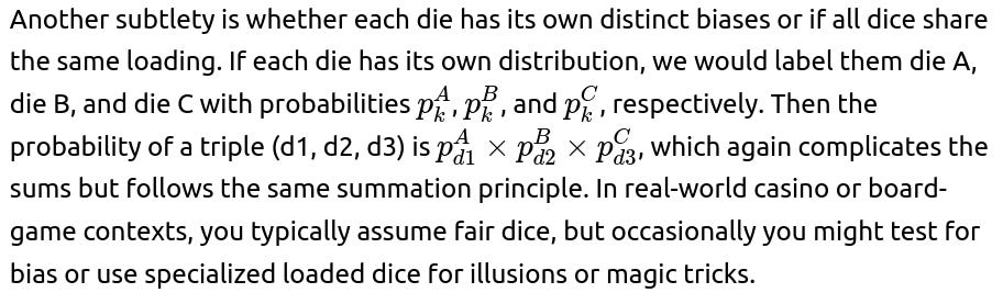
If each die face does not have the same probability of occurring, the uniform assumption breaks. The straightforward counting method of equally likely outcomes (216 total ordered outcomes, 120 with distinct faces, and so on) no longer holds. Instead, each triple of outcomes (d1, d2, d3) has a probability that depends on the product of the probabilities of each face for each die.

To find the probability that the dice are all distinct, one would sum the above term over all distinct triples (d1, d2, d3). Similarly, to find the probability of summing to 12 and having all distinct faces, one would sum only over those (d1, d2, d3) for which d1 + d2 + d3 = 12 and d1, d2, d3 are pairwise different. The conditional probability then becomes:

A key pitfall is that if one tries to use a counting approach (like 18 out of 120) and multiplies by some weighting factor, it may lead to an incorrect answer unless the non-uniform probabilities maintain the exact same ratio across all distinct triples. In reality, distinct faces that involve high-probability faces (like if 6 has a very high bias) become disproportionately more likely. Thus, you cannot rely on simple integer counting; you must incorporate the actual probability distribution of each face.

How would the result differ if the dice were considered indistinguishable?

When dice are considered indistinguishable (unlabeled), the sample space changes dramatically. In the indistinguishable case, the outcome is not an ordered triple (d1, d2, d3), but rather a combination with repetition allowed. For example, the outcome “(1,2,3)” would be the same as “(3,2,1)” or “(2,1,3)” because the dice are not labeled. You can represent such outcomes with partitions or multisets.

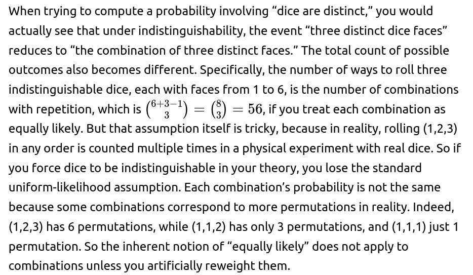
Hence, the biggest pitfall is ignoring that real dice are inherently labeled in practice (the first, second, and third roll are distinct events). If you artificially treat them as indistinguishable, you must track how many permutations map to the same combination. Otherwise, you will compute the wrong probability. This is often a subtle conceptual difference that can trip up even experienced mathematicians in more complicated scenarios.

Could the events “sum = 12” and “dice are distinct” ever be independent?

The events “sum = 12” and “dice are distinct” are not independent. Independence would require:

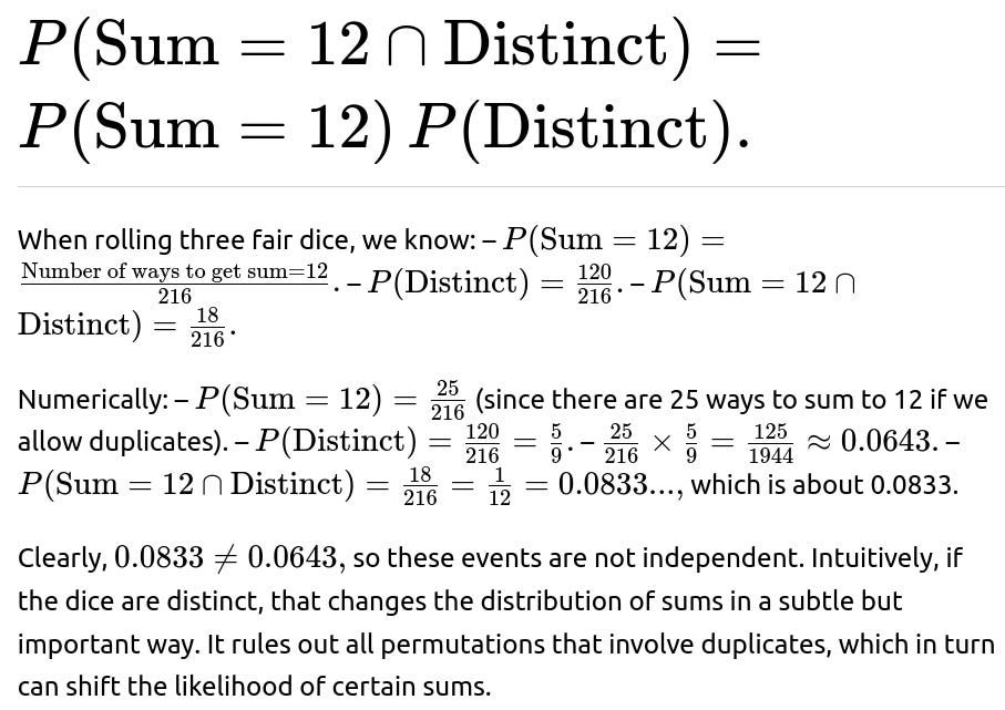
In a more general sense, for an event to be independent of “dice are distinct,” it would mean that the likelihood of that event is not affected by whether we know the dice are distinct or not. But sums that require or are more easily composed with duplicates (like sum = 18 requires all three dice to be 6) are obviously heavily affected by the distinctness condition, so independence does not hold for any sum except in contrived or degenerate dice scenarios.

What if we introduced a fourth die and still asked for a similar conditional probability?

If four fair six-sided dice are rolled, and you want the probability that they sum to some value (for instance, 12, but now it’s a different distribution) given that all four are distinct, you would repeat a process analogous to the original approach but with an expanded sample space.

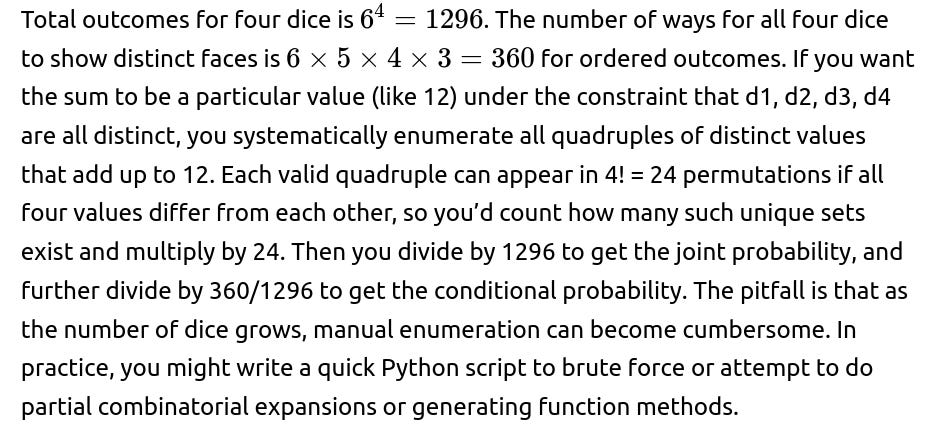
Edge cases appear if you let the sum approach extremes. For four dice, the minimum sum is 4 and the maximum sum is 24. Some sums can’t be reached by distinct faces alone (for example, sum=24 requires all four dice to be 6, which is not distinct). This ensures some sums have zero probability under the distinctness condition. Similarly, sums closer to the extremes can often require duplicates, so they become less likely (or impossible) when the dice are forced to be distinct. All of that can shift probabilities drastically.

How can sampling or simulation lead to errors if not carefully done?

To estimate this probability by simulation, you might write a simple Python or C++ script to roll three virtual dice many times, filter only the trials in which all dice are different, and among those, estimate how often the sum is 12. While this Monte Carlo approach should converge to the true probability with enough trials, several pitfalls can arise.

One pitfall is pseudo-random number generation issues, such as poorly seeded or correlated random draws. Another is failing to track the distinct condition properly, for instance, incorrectly ignoring or not ignoring trials that contain duplicates. Also, if the number of trials is too small, random fluctuation can yield a biased result. For example, if you do only a few thousand trials, you might see fairly large confidence intervals around your estimate.

A further subtlety is mixing up the logic in the code. If you compute the probability that “sum = 12” and “dice are distinct” in separate loops or you filter data incorrectly, you can get the wrong conditional probability. You must be consistent: among all the rolls that produced distinct values, check how many of those produce a sum of 12, and then divide. Observers sometimes make the mistake of first restricting to sum=12 outcomes and then trying to see how many are distinct, which is valid only if you also track the correct denominator. Another simple error is forgetting to cast to float in languages like C++ or Python 2, which can lead to integer division issues.

How would the result be impacted if one of the dice was guaranteed to be a certain value?

Suppose you know in advance that the first die is definitely a 4 (maybe you physically see it land first or it’s rigged to always be 4), and you still want “sum=12 given the three dice are distinct.” In that scenario, effectively the first die is no longer random for the sum. You have two random dice plus that known 4. The sum condition is “(4 + d2 + d3) = 12,” so “d2 + d3 = 8,” and you also want d2, d3 both distinct from 4 and from each other.

Counting outcomes changes in a fairly direct manner:

For distinctness: – The second die can take values in {1,2,3,5,6} because it cannot be 4. – The third die can take values in {1,2,3,5,6} minus whichever the second die took, so 4 possible distinct values remain.

Hence 5 × 4 = 20 total ways to have the second and third dice distinct from each other and from the first die of 4. Among those 20, how many sum to 8? You can list pairs for (d2, d3) in {1,2,3,5,6} such that d2 + d3 = 8 and d2 ≠ d3, and neither is 4. For example (3,5) or (5,3) or (2,6) or (6,2). This yields 4 valid ordered pairs. So the conditional probability that the second and third dice sum to 8 among the 20 distinct pairs is 4/20 = 1/5. This is quite different from the unconditional scenario of “three fair dice all distinct.” The shift results from the prior knowledge that the first die is pinned to 4 and is automatically distinct from the others.

This kind of scenario highlights how prior or partial knowledge (one outcome is known or constrained) can change the sample space drastically. If the first die is pinned to a 4 that might or might not be fair, you also have to factor in that die’s probability distribution if you were analyzing from a more general Bayesian perspective. But from a purely conditional approach, you just recast the problem as two dice needing to sum to 8 while being distinct from each other and from 4.

How would you use Bayes’ Theorem if you had partial knowledge of the sum?

Bayes’ Theorem can be relevant if you observe partial outcomes or partial sums and want to infer the likelihood of distinctness. For example, imagine you know the sum is 12 or more, and you want to compute the probability that the dice are distinct given that sum≥12. Then you would frame:

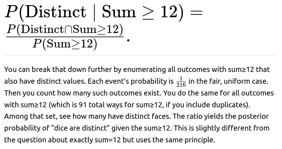
A key pitfall is forgetting that “sum≥12” includes sums of 12, 13, 14, …, 18. Some of those sums might heavily rely on repeated faces (like sum=18 requires three 6s, which is obviously not distinct). Others can easily be formed by distinct faces. If you ignore or miscount the combinations that produce sums greater than 12 with duplicates, you can incorrectly inflate or deflate the final ratio.

Bayes’ Theorem is particularly helpful in scenarios where you want to invert the direction of a known conditional probability. For instance, you might know “if the dice are distinct, the sum=12 has probability 3/20,” and you want “if the sum=12, the dice are distinct with some probability.” In that latter direction, you would compute:

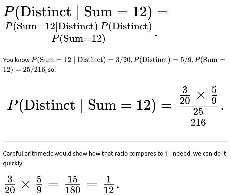
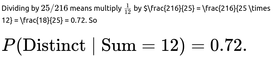
Hence, if you see that the sum is 12, there is a 72% chance that all dice are distinct. This is interestingly higher than 50%, reflecting the fact that duplicates or triplicates (like two 6s and a 0, which is not possible, or three 4s, which sums to 12 only if it’s 4+4+4=12 but that’s not distinct) are somewhat less likely. If you do not keep the numbers straight, you can easily slip up in applying Bayes’ Theorem.

Would the probability change if we used dice with different side sets, like a trick die that has faces 1,1,2,2,3,6?

If you had a peculiar or trick die that does not contain the typical faces {1,2,3,4,5,6} but instead has repeated or altered faces, then even the sample space for that single die changes. For instance, if a trick die has faces {1,1,2,2,3,6}, it does not have 4 or 5, and it duplicates 1 and 2. The sums you can form with three such dice (or some combination of standard dice and trick dice) would differ from the standard scenario. The distinctness condition might also be partially or entirely moot if the trick die cannot produce some faces at all or can produce repeated faces with different probabilities.

You would handle this systematically by enumerating all possible faces each die can show (with the correct probability for each face), ensuring you track which faces are even feasible. The distinctness constraint would require (d1, d2, d3) all be different, but if your trick die can only show {1,1,2,2,3,6}, then effectively it can show 1 with probability 2/6, 2 with probability 2/6, 3 with probability 1/6, and 6 with probability 1/6. If you have three identical trick dice or some combination with standard dice, you multiply out the probabilities for each triple. For example:

If you have 3 identical trick dice, each triple (d1, d2, d3) has probability:

but you must verify that distinctness is even possible for certain faces. If the dice can only produce 1, 2, 3, 6 in general, you might see that some sums (like sum=12) become more or less probable because 4 and 5 are not possible on any single die. Also, you might find there are fewer distinct ways to get certain sums, or some sums can’t be formed while preserving distinctness.

The pitfall is that you cannot rely on standard formulas like 6 × 5 × 4 = 120 for distinct faces because it might not even be possible to choose three distinct faces if the trick die only has a limited set. You must carefully map out every possible triple. Real-world illusions or specialized dice might use such distributions to create illusions of randomness or to cheat at certain games. If an interviewer asks you about them, they want to see if you can adapt your approach away from the default assumption that each die is a fair six-sided device with faces {1,2,3,4,5,6}.

How does this connect to the concept of random variables and distributions more abstractly?

Each die roll can be thought of as a discrete random variable X, taking values in {1,2,3,4,5,6} with probability 1/6 in the fair case. Then for three dice, you have X1, X2, X3, each representing a roll. The event “dice are distinct” is:

We can define a new random variable S = X1 + X2 + X3. Probability statements like “P(S=12∣all distinct)” are standard conditional probability statements in the space of (X1, X2, X3). From a distribution perspective, S is the convolution of three i.i.d. discrete uniform distributions. The distinctness condition is a constraint that shapes the sample space. Conceptually, it is a standard demonstration of how restricting a sample space can alter the relative likelihoods of different events.

In advanced probability or data science contexts, one might sample from or manipulate distributions with complicated dependencies or constraints. The principle remains: you either do a direct combinatorial count or you sum/integrate the probability mass or density over the region that satisfies your condition. The tricky bits often lie in making sure you have enumerated or integrated correctly, respecting both the desired event (sum=12) and the condition (dice are distinct).

Pitfalls occur if you try to treat these dice variables as independent after imposing a “distinctness” condition, which actually introduces a dependence among X1, X2, and X3. For instance, if you know X1=2, that changes the probability distribution of X2 if you are conditioning on them being distinct. So it is no longer correct to treat X2 as uniform in {1,2,3,4,5,6} under that condition. That can lead to errors if you blindly multiply probabilities as though they remain independent.

How would you extend this reasoning to build a distribution or table for all sums and the number of distinct faces?

One interesting extension is to create a joint distribution table for the pair of random variables:

– S, the sum of the three dice, taking values from 3 to 18. – D, the number of distinct faces, which can be 1, 2, or 3 for three dice.

Then you’d fill out a 16 × 3 table (sums 3 through 18, and distinctness levels 1, 2, 3) with probabilities or counts. For instance, (S=12, D=3) has a count of 18, (S=12, D=2) might be all permutations of (6,6,0) which is impossible because the faces must be between 1 and 6, so you’d systematically count valid sets. Actually, for S=12 and D=2, we can think about (5,5,2), (4,4,4) is D=1, so you’d carefully find how many ways get S=12 with exactly two distinct faces, how many ways get S=12 with exactly one distinct face (which is 4,4,4, only 1 way out of 216). By enumerating for each sum from 3 to 18, you get a complete picture. From that table, you can read off any conditional probability you want: for example, “Given S=12, what is P(D=3)?” (which is precisely the probability that the dice are distinct given sum=12). You can do the same for any sum or any distinctness count.

This approach teaches you systematically to handle events that cut across multiple random variables. The pitfall is the complexity of building such a table by hand. One might do it with a program that systematically loops over (d1, d2, d3) in the range [1..6] × [1..6] × [1..6], counts each sum, counts how many distinct faces are in that triple, and records it. From there, you can produce the joint distribution. That’s more systematic and less prone to small mistakes like missing a triplet that sums to 12.

How is the concept of “hypergeometric” or “inclusion-exclusion” relevant here?

For the event “dice are distinct,” one might consider inclusion-exclusion if you are dealing with sets or if you tried to approach it from a combinatorial formula perspective:

P(dice are distinct)=1−P(at least two dice are the same).

But enumerating or calculating P(at least two dice are the same) can get tricky with events like “d1 = d2,” “d2 = d3,” “d1 = d3.” In principle:

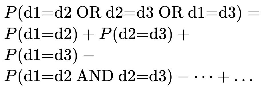
This inclusion-exclusion quickly becomes a bit messy for a small problem. It’s simpler to do direct counting for three dice. However, for more complex or generalized problems (like 10 dice, each with 6 sides, or dice with more sides), you might need an inclusion-exclusion approach if you want an exact closed-form expression.

Similarly, a hypergeometric perspective arises in certain problems of drawing without replacement. If you consider rolling dice with the constraint that no face can appear more than once, you’re effectively sampling from the set {1,2,3,4,5,6} without replacement. However, the major difference is that dice rolling is typically “with replacement” from the set {1..6} for each roll. So hypergeometric might be more relevant if you physically had a box with the numbers 1 through 6 on slips of paper, and each draw was a distinct slip. Then you’d never see the same face repeated. But that’s not normal dice rolling. Real dice rolling is more akin to binomial or multinomial sampling with replacement (each roll is an independent pick from {1..6}), so hypergeometric is not the usual tool for standard dice problems. The pitfall is to incorrectly treat standard dice rolling as though it were hypergeometric sampling from a set of 6 numbers.

What special care should we take if we scale up to many dice and are asked about the probability that all dice are distinct?

If you scale up to n dice, each with 6 faces, eventually you cannot have all dice distinct if n>6 because you cannot choose more than 6 distinct values from a set of 6. So for n>6, the probability that all dice are distinct is zero. Even for n=6, the only way all dice can be distinct is to permute the faces 1 through 6 in some ordering, so you would have 6! = 720 ways out of 6^6 = 46656 total. That yields 720/46656≈0.0154 or 1.54%.

For n<6, you can do a combinatorial approach:

The probability that all n dice are distinct =

Then if you want the probability of a particular sum (like 12) under that constraint, you would again combine an enumeration or formula for the sum distribution with the distinctness restriction. The pitfall, of course, is that for large n, enumerating sums is extremely tedious, and generating functions or dynamic programming might be your best approach. Another subtlety is that as n grows, you have to keep in mind that if n>6, the probability of being distinct is zero, and that makes many conditional probabilities either undefined or zero, so you have to handle that carefully in code or in theoretical expressions.

How might you validate these probabilities in an interview without memorizing them?

In an interview, you could show how you would quickly set up a brute-force enumeration or explain a combinatorial argument. For example, you might say:

You would write a short snippet of Python that loops over d1 in [1..6], d2 in [1..6], d3 in [1..6], counts how many times (d1+d2+d3=12) and how many times all dice are distinct, etc. Then you would do your ratio. If pressed for time, you might do partial enumerations by logic (like we do for sum=12: (1,5,6), (2,4,6), (3,4,5), each with 6 permutations) to demonstrate that you understand the distinct permutations. The final answer of 3/20 emerges swiftly if you trust your counting. But you reassure the interviewer that if there was any doubt, you’d run a quick simulation or code snippet to confirm. That kind of approach—double-checking your theoretical results with a quick coded experiment—often impresses technical interviewers because it shows you can shift between theory and practice.