
ML Interview Q Series: Conditional Densities & Expectations for Uniform Variables Given U1 > U2

Browse all the Probability Interview Questions here.
Let U1 and U2 be two independent random variables that are uniformly distributed on (0,1). How would you define the conditional densities of U1 and U2 given that U1 > U2? What are E(U1 | U1 > U2) and E(U2 | U1 > U2)?
Short Compact solution
We first note that P(U1 > U2) = 1/2. Then for any 0 ≤ x ≤ 1:
The conditional cumulative distribution function of U1 given U1 > U2 is: P(U1 ≤ x | U1 > U2) = x², so differentiating gives the conditional density 2x for 0 < x < 1.
The conditional cumulative distribution function of U2 given U1 > U2 is: P(U2 ≤ x | U1 > U2) = 2(x - x²/2) = 2x - x², so differentiating gives the conditional density 2(1 - x) for 0 < x < 1.
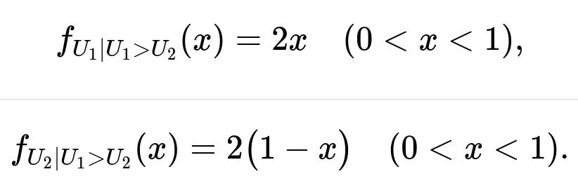
Hence the conditional densities are:
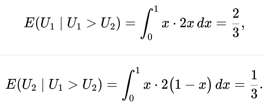
Their conditional expectations then follow by computing the integrals:
Comprehensive Explanation
The reasoning behind the conditional densities
U1 and U2 are i.i.d. (independent and identically distributed) uniform(0,1). The event U1 > U2 occurs with probability 1/2, because symmetry ensures that P(U1 > U2) = P(U2 > U1) = 1/2.
To find f_{U_1 | U_1 > U_2}(x), we look at:
P(U1 ≤ x | U1 > U2).
By definition,
P(U1 ≤ x | U1 > U2) = [P(U1 ≤ x, U1 > U2)] / P(U1 > U2).
We can compute P(U1 ≤ x, U1 > U2) by integrating over the region where 0 < u2 < u1 ≤ x:
∫(u1=0 to x) ∫(u2=0 to u1) (1) du2 du1,
since U1, U2 ~ uniform(0,1) implies joint density 1 for 0 < u1, u2 < 1. Dividing by P(U1 > U2) = 1/2, we get:
[∫(0 to x) ∫(0 to u1) 1 du2 du1] / (1/2).
The inner integral ∫(0 to u1) 1 du2 = u1, and then the outer integral becomes ∫(0 to x) u1 du1 = x²/2. After dividing by 1/2, we get x². Thus:
P(U1 ≤ x | U1 > U2) = x².
Differentiating x² w.r.t. x gives 2x, so
f_{U_1 | U_1 > U_2}(x) = 2x, for 0 < x < 1.
By a similar argument:
P(U2 ≤ x | U1 > U2) = [P(U2 ≤ x, U1 > U2)] / P(U1 > U2).
This is the region 0 < u2 ≤ x < 1 and u1 > u2. In terms of integrals:
∫(u2=0 to x) ∫(u1=u2 to 1) 1 du1 du2,
and then we divide by 1/2. The inner integral ∫(u1=u2 to 1) 1 du1 = 1 - u2, so
∫(u2=0 to x) (1 - u2) du2 = x - x²/2.
Dividing by 1/2 yields 2(x - x²/2) = 2x - x². Differentiating this w.r.t. x gives 2(1 - x), so
f_{U_2 | U_1 > U_2}(x) = 2(1 - x), for 0 < x < 1.
Deriving the conditional expectations
With the conditional densities in hand:
E(U1 | U1 > U2):
We use ∫(0 to 1) x * (2x) dx, because f_{U_1|U_1>U_2}(x) = 2x for 0 < x < 1. Evaluating:
∫(0 to 1) 2x² dx = 2 * (1/3) = 2/3.
E(U2 | U1 > U2):
We use ∫(0 to 1) x * (2(1 - x)) dx, because f_{U_2|U_1>U_2}(x) = 2(1 - x) for 0 < x < 1. Evaluating:
∫(0 to 1) 2x(1 - x) dx = 2 * ∫(0 to 1) (x - x²) dx = 2 * [(1/2) - (1/3)] = 2 * (1/6) = 1/3.
Hence,
E(U1 | U1 > U2) = 2/3 and E(U2 | U1 > U2) = 1/3.
Intuitive interpretation
The condition U1 > U2 skews U1 to be “larger” on average and U2 to be “smaller.” Because of uniform(0,1) symmetry, you might expect the midpoint of the region where U1 > U2 is biased such that U1’s average is 2/3 while U2’s average is 1/3 in that region.
Potential Follow-Up Questions
Why does P(U1 > U2) = 1/2?
Since U1 and U2 are independent uniform(0,1), each ordering (U1 > U2 or U2 > U1) is equally likely. Another way is to compute:
P(U1 > U2) = ∫(0 to 1) ∫(0 to u1) 1 du2 du1 = 1/2.
Could you have deduced E(U1 | U1 > U2) without computing the entire conditional distribution?
Yes. One alternative approach uses symmetry arguments and the “order statistics” viewpoint. If we consider two i.i.d. uniform(0,1) variables, the event U1 > U2 is equivalent to saying “U1 is the maximum and U2 is the minimum.” For two i.i.d. uniform(0,1), the expected maximum is 2/3 and the expected minimum is 1/3. Hence, conditioned on U1 being the larger one, U1’s expectation must be 2/3 and U2’s expectation must be 1/3.
How do these results generalize to multiple uniform random variables?
For N i.i.d. uniform(0,1) variables, the expected k-th order statistic is k/(N+1). In the case N=2, the larger one is the second order statistic whose mean is 2/(2+1) = 2/3, and the smaller one is the first order statistic with mean 1/(2+1) = 1/3.
How would you simulate this in Python?
You could generate many samples of U1 and U2 from uniform(0,1), keep only those pairs where U1 > U2, and then average U1 and U2 values in that subset. A quick demonstration:
import numpy as np

num_samples = 10_000_000
U1 = np.random.rand(num_samples)
U2 = np.random.rand(num_samples)

mask = U1 > U2
U1_conditioned = U1[mask]
U2_conditioned = U2[mask]

print("Estimated E(U1 | U1>U2):", np.mean(U1_conditioned))
print("Estimated E(U2 | U1>U2):", np.mean(U2_conditioned))
With sufficiently large num_samples, you will see estimates around 0.666... for E(U1|U1>U2) and around 0.333... for E(U2|U1>U2).
What if U1 and U2 were not uniform(0,1)?
The derivation would differ, because their joint density over the domain would not be constant. You would compute:
P(U1 ≤ x | U1 > U2) = [∫(u1=0 to x) ∫(u2=0 to u1) f_{U1,U2}(u1,u2) du2 du1] / P(U1 > U2),
where f_{U1,U2}(u1,u2) is their joint pdf. Similarly, you would proceed for U2. In general, the integrals become more complicated, and the resulting conditional pdf might not take a simple closed form.
How would you handle discrete random variables in a similar problem?
For discrete random variables X and Y, you would consider:
P(X = x | X > Y) = P(X = x, X > Y) / P(X > Y).
You would sum over all y such that y < x, specifically:
P(X = x | X > Y) = [Σ over y < x of P(X = x, Y = y)] / P(X > Y).
Hence, you would adapt the continuous approach to a summation approach. The concept remains the same: you restrict to the event X > Y and renormalize.
These details (continuous vs discrete) illustrate how the fundamental idea of conditional probability remains consistent, but the integrals become sums for discrete cases, and the distribution shapes differ depending on the original distribution assumptions.
Below are additional follow-up questions
What happens at the boundaries x=0 and x=1 for the conditional densities?
The conditional density functions f_{U1|U1>U2}(x)=2x and f_{U2|U1>U2}(x)=2(1−x) are each defined strictly for 0 < x < 1. At x=0 or x=1, these density values are not strictly positive, and we typically treat them as 0 in the continuous setting because the probability that U1 or U2 is exactly 0 or 1 in a uniform(0,1) distribution is 0. In other words:
At x=0, 2x=0, so the density goes to zero. Intuitively, the chance that U1 is exactly at 0 while also exceeding U2 is effectively null.
At x=1, 2(1−x)=0, so the density for U2 given U1>U2 also goes to zero as x approaches 1.
Pitfall/Edge case: If someone tries to integrate from 0 to 1 without carefully specifying the density at boundaries, they might worry about whether the functions are well-defined. However, for continuous distributions, any single point has probability 0, so the density can be safely taken as 0 at the boundary with no impact on integrals.
How would the situation change if the domain of (U1, U2) were not (0,1) but some general interval (a, b)?
If U1 and U2 are i.i.d. uniform(a, b), then P(U1>U2) is still 1/2. The conditioning event U1>U2 partitions the square [a,b]×[a,b] into two equal triangles. However, the integrals become:
For f_{U1|U1>U2}(x), you would compute P(U1 ≤ x, U1>U2) / P(U1>U2) within [a,b].
After rescaling, you’d find that the forms of the conditional densities are analogous, but shifted and scaled over [a,b]. We expect E(U1|U1>U2) to be a number in (a,b), specifically a linear shift from 2/3 in the original (0,1) case. Indeed, one can show that the result will be (2/3)(b−a)+a and similarly (1/3)(b−a)+a for U2.
Pitfall/Edge case: For (a,b) with a≠0 or b≠1, failing to incorporate the shift and scaling can cause confusion. Some might incorrectly assume the integrals remain the same as (0,1) without adjusting the limits or the uniform density value, which is 1/(b−a) rather than 1.
What if U1 and U2 follow some mixed distribution, partly discrete and partly continuous?
In a mixed distribution scenario, the joint distribution is partly discrete mass at certain points or intervals and partly continuous on others. To find P(U1>U2), you would sum/integrate over all combinations of those discrete and continuous regions. Then the conditional density would be derived by restricting to U1>U2 and renormalizing within that subset of the mixed domain. The final f_{U1|U1>U2} and f_{U2|U1>U2} might be piecewise functions with point masses and/or continuous segments.
Pitfall/Edge case: A common mistake is to overlook the contribution from the discrete portion. You must explicitly account for the probability mass at discrete values. If there is a chance that either variable can take exact values with positive probability, you must handle those points carefully in the conditioning event U1>U2.
How would rounding or finite precision in real-world data affect the result?
In practical computing contexts, uniform(0,1) variables might be quantized to floating-point precision. This effectively introduces a minor discrete aspect at very fine resolution. The condition U1>U2 could become tricky near boundaries or if U1≈U2, because numerical floating-point comparisons can yield unexpected outcomes when values are nearly identical. Over many samples, the effect is typically small, but it can shift the empirical probability that U1>U2 slightly away from 1/2.
Pitfall/Edge case: If the data are heavily rounded (e.g., a random number generator that only produces discrete steps of 0.001), the theoretical integrals might deviate from the empirical results. This can be critical in high-precision simulations where verifying your random generator’s uniformity or dealing with potential ties is important.
What if U1 ≥ U2 (allowing equality) rather than strictly U1 > U2?
Allowing U1=U2 with nonzero probability under a continuous distribution does not matter in theory because P(U1=U2)=0 for continuous i.i.d. uniform(0,1). But if the specification changes to ≥, it typically makes no difference in the continuous case because the set {U1=U2} is measure zero. In a discrete or finite-precision setting, however, U1=U2 might have a small non-negligible probability.
Pitfall/Edge case: In discrete or quasi-discrete approximations, the event U1=U2 can have positive probability. In that scenario, the difference between “>” and “≥” can matter. For instance, if you are dealing with integer values from 0 to 100, you need to decide how to treat the probability mass when U1=U2.
How would you handle the scenario where U1 and U2 are correlated?
The derivation depends on the joint density being factorable as f_{U1,U2}(u1,u2)=f_{U1}(u1)f_{U2}(u2). If U1 and U2 are correlated, then:
P(U1>U2) is no longer 1/2 in general.
The region where U1>U2 must be integrated with the joint density f_{U1,U2}(u1,u2).
You would then form f_{U1|U1>U2}(x)=P(U1=x and U1>U2)/P(U1>U2), but in continuous form it requires a proper integral with the correct correlation structure.
Pitfall/Edge case: A naive approach is to assume the unconditional uniform marginals and then incorrectly keep P(U1>U2)=1/2. Correlation can shift that probability significantly. For example, if U1 and U2 have positive correlation, U1>U2 might occur less or more frequently than 1/2, depending on their joint dependency structure.
How do the results generalize to random variables that are not identically distributed?
If U1 ~ uniform(0,1) and U2 ~ uniform(0,2), for instance, they do not have the same distribution, and the symmetry is broken. You must compute: P(U1>U2)=∫ ∫ (region where u1>u2) f_{U1}(u1) f_{U2}(u2) du2 du1, and similarly the conditional pdf f_{U1|U1>U2}(x). The conditional expectations will be different from 2/3 and 1/3. Each integral must reflect the correct marginal densities.
Pitfall/Edge case: One might attempt to use order-statistic shortcuts or symmetry arguments that only apply to i.i.d. cases. With non-identical distributions, the standard 2/3 and 1/3 do not hold, so you must do the exact integration.
What if you want to estimate these conditional expectations from real data (observed pairs of (U1, U2)) rather than from a known distribution?
In real-world data collection, you might have samples of (U1, U2) (e.g., two measured quantities). You want E(U1|U1>U2). The approach is:
Filter the dataset to include only cases where U1>U2.
Compute the average of U1 in that filtered dataset as an empirical estimator of E(U1|U1>U2).
Similarly for U2.
Pitfall/Edge case: If you have limited data, the subset where U1>U2 could be small, so variance in your estimator might be large. Also, if the data are not truly uniform(0,1) or are correlated, the theoretical result does not match the empirical. You must ensure your data truly follow the model assumptions, or else use a more general approach like kernel density estimation to approximate the joint density and then condition.
How can you visualize the event U1>U2 to confirm these calculations?
You can plot the unit square [0,1]×[0,1] with the region U1>U2 (the set of points above the diagonal line u1=u2). Under uniform(0,1), the joint pdf is flat, so the probability corresponds to the area above the diagonal line, which is 1/2. Likewise, you can overlay the density for U1 or U2 restricted to that region. A 3D surface plot or a heatmap can highlight how U1 is more likely to be larger within that region, consistent with the derived densities.
Pitfall/Edge case: If your distribution were not uniform, the region of integration in [0,1]×[0,1] might have a different shape or weighting, so the graphical intuition must incorporate the actual joint pdf. Relying on geometry alone might overlook the effect of a non-constant density.
In a small-sample simulation or experiment, how do you judge if the observed E(U1|U1>U2) significantly differs from 2/3 due to randomness?
You can construct confidence intervals around the sample mean. For n i.i.d. draws of (U1, U2), the number of draws where U1>U2 is roughly n/2 in expectation. From that subsample, you can compute the sample mean of U1 and use standard error calculations (assuming i.i.d. samples). You might approximate:
Std. Error ≈ (sample std. dev. of U1 in that subset) / sqrt(number of U1>U2 cases).
Pitfall/Edge case: If n is small, or if the data are not truly uniform(0,1), or if there is correlation, the standard normal approximation might be inaccurate. Bootstrap methods can be used instead, resampling from the dataset to get a more robust confidence interval.