
ML Interview Q Series: Conditional Binomials: Joint PMF and P(X=Y) for Die-Driven Coin Flips

Browse all the Probability Interview Questions here.
Roll a fair die once. Let N be the outcome of this roll. Then two persons toss each N fair coins, independently of each other. Let X be the number of heads obtained by the first person and Y be the number of heads obtained by the second person. What is the joint probability mass function of X and Y? What is the numerical value of P(X = Y)?
Short Compact solution
The joint probability mass function (pmf) is obtained by conditioning on the die outcome N = n, which occurs with probability 1/6 for n in {1, 2, 3, 4, 5, 6}. Given N = n, each person’s number of heads follows a Binomial(n, 1/2) distribution independently. Summing over all possible n yields:
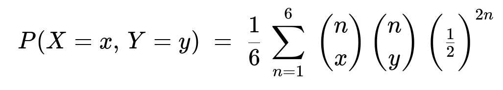
where (n choose x) = 0 whenever x > n or x < 0, and similarly for y.
For the probability P(X = Y), one uses the identity sum_{k=0..n} (n choose k)^2 = (2n choose n). Thus:

Comprehensive Explanation
Derivation of the Joint pmf
Conditional on the die outcome (N = n) When the fair die shows n, each person tosses n fair coins. The number of heads for the first person X (given N = n) follows a Binomial(n, 1/2) distribution. Independently, Y (given N = n) also follows a Binomial(n, 1/2) distribution. Hence:
P(X = x, Y = y | N = n) = [ (n choose x) (1/2)^n ] * [ (n choose y) (1/2)^n ] for 0 <= x, y <= n.
Accounting for the probability of N Because the die is fair, P(N = n) = 1/6 for n in {1, 2, 3, 4, 5, 6}. So by the Law of Total Probability:
P(X = x, Y = y) = sum_{n=1..6} [ P(N = n) * P(X = x, Y = y | N = n) ]. Substituting:
P(X = x, Y = y) = (1/6) sum_{n=1..6} [ (n choose x)(1/2)^n * (n choose y)(1/2)^n ] = (1/6) sum_{n=1..6} (n choose x)(n choose y)(1/2)^(2n).
Handling the range of x and y For x, y in {0, 1, 2, …, 6}, note that (n choose x) = 0 whenever x > n or x < 0, so effectively in the summation only terms for which x <= n and y <= n contribute nonzero values.
Derivation of P(X = Y)
Set X = Y = k To find P(X = Y), one can sum over all k in {0, 1, 2, …} but in practice k is bounded because the maximum number of heads is 6. Formally:
P(X = Y) = sum_{x=0..6} P(X = x, Y = x).
Expressing it in terms of n Condition on N again:
P(X = Y) = (1/6) sum_{n=1..6} sum_{k=0..n} (n choose k)^2 (1/2)^(2n).
Using the combinatorial identity The key identity is sum_{k=0..n} (n choose k)^2 = (2n choose n). This simplifies the inner sum:
sum_{k=0..n} (n choose k)^2 = (2n choose n).
Hence:
P(X = Y) = (1/6) sum_{n=1..6} (2n choose n) (1/2)^(2n).
Evaluating this sum numerically yields approximately 0.3221.
Why the Combinatorial Identity Holds
For completeness: sum_{k=0..n} (n choose k)^2 = (2n choose n) stems from interpreting (n choose k)(n choose n-k) in a combinatorial argument of choosing n objects from 2n, or via the binomial coefficient expansions in more advanced algebraic proofs.
Relationship Between X and Y
It is important to note that although X and Y are conditionally independent given N (because each person’s coin tosses are independent once N is fixed), X and Y are not marginally independent without conditioning on N. The reason is that both X and Y depend on the common random variable N. If you observe a large value of X, that makes it slightly more likely that N was large, which in turn influences the distribution of Y.
Example Calculation in Python
Below is a simple Python snippet to compute P(X=Y) directly by enumerating over all possible n, x, y. This can verify the numeric result of approximately 0.3221.
import math

def choose(n, k):
    return math.comb(n, k)  # Python 3.8+

p_equal = 0
for n in range(1, 7):
    for k in range(n+1):
        p_equal += (1/6) * choose(n, k)**2 * (1/2)**(2*n)

print(p_equal)  # ~ 0.3221
Potential Follow-up Questions
Are X and Y independent?
No, they are not independent in the marginal sense. Even though X and Y are conditionally independent given N, the distribution of (X, Y) when N is unobserved introduces dependence. Observing X can give some information about N, which in turn influences the likely range of Y.
What if the die is unfair?
If P(N = n) is not uniform, we would simply replace the factor 1/6 with P(N = n). Then:
P(X = x, Y = y) = sum_{n=1..6} [ P(N = n) * P(X = x, Y = y | N = n) ].
Everything else in the binomial terms remains the same, but the final sums would be weighted by the different probabilities of N.
What if the coins are biased with probability p instead of 1/2?
For a fixed N = n, X ~ Binomial(n, p) and Y ~ Binomial(n, p) independently. The overall pmf becomes:
P(X = x, Y = y | N = n) = (n choose x) p^x (1 - p)^(n - x) * (n choose y) p^y (1 - p)^(n - y).
Summing over n yields:
P(X = x, Y = y) = sum_{n=1..6} [ P(N = n) * (n choose x) p^x (1 - p)^(n - x) * (n choose y) p^y (1 - p)^(n - y) ].
The computation for P(X = Y) requires a more general identity (or direct summation), and the numeric value changes accordingly.
Could we have simplified the computation of P(X=Y) by another approach?
Yes. One might attempt to use generating functions or moment generating functions. But the combinatorial identity is very direct. Alternatively, summation by direct enumeration (as in the Python snippet) is often straightforward for a small range of n.
How to interpret this scenario in real-world settings?
Multiple stages of randomness: N is chosen first (the die roll), and then X, Y are drawn from a binomial with parameter depending on N. This sort of hierarchical setup appears frequently in random processes with multiple steps (e.g., random numbers of trials in different experiments).
Conditional vs. marginal distributions: Understanding the difference between conditional independence (given N) and marginal dependence is crucial in real-world applications, especially in Bayesian modeling contexts or hierarchical modeling frameworks.
Extending to more persons: If more persons each tossed N coins, all their numbers of heads would be conditionally independent given N but remain marginally dependent.
These points often arise in modeling real-world processes where the total number of “opportunities” or “trials” is itself random, and then the number of “successes” in each trial depends on that total.
Below are additional follow-up questions
What if the die could show zero (N=0)? How does that affect the distribution?
If there is a nonzero probability that N=0 (a degenerate or modified die scenario), then with probability P(N=0), neither person tosses any coins. In that case X and Y would both be forced to be zero with probability 1 for that part of the mixture. Formally, when N=0, P(X=0, Y=0 | N=0) = 1, and for X≠0 or Y≠0, the probability is 0. This would add a term to the overall mixture in the joint pmf:
P(X=x, Y=y) = P(N=0) · [1 if (x=0, y=0) else 0] + sum over n>0 of [ P(N=n) · binomial-terms ].
A subtlety arises if the problem statement originally implied N≥1 by definition, but if someone modifies the die or includes zero in the outcome space, we must adjust the domain of n accordingly and incorporate that “no coin toss” scenario in the mixture. This situation can occur in real-world processes where a “trial count” can be zero, forcing all outcomes of interest to be zero.
What if X or Y exceeds 6 in the final distribution?
Under normal circumstances, X or Y cannot exceed 6 because N can only be as large as 6. Consequently, for x>6 or y>6, the joint pmf is 0. However, if we were to allow N to be larger than 6 (for example, an n-sided die with n>6), then we must adjust the summation range accordingly. As soon as the maximum possible N grows, the support for X and Y grows as well, and the binomial terms would accommodate larger x and y. In a real implementation, failing to clip x and y at the relevant maximum can lead to coding errors—like trying to evaluate (n choose x) for x>n—which is 0 by definition, but must be handled carefully to avoid out-of-range or computational mistakes.
Is the distribution of (X, Y) symmetric in X and Y?
Yes, the distribution is symmetric in X and Y because each person tosses the same number of coins (N) with the same bias (1/2), independently. Mathematically, the formula for P(X=x, Y=y) is unchanged if we swap x and y. This symmetry also shows up in the fact that P(X=Y) = P(Y=X). Potential pitfalls might arise in a scenario where someone tries to impose additional constraints making the second person’s tosses not identically distributed (for instance, different coin bias or a different count of coin tosses). In that case, symmetry would no longer hold.
How would one analyze the distribution of the difference X - Y?
The random variable X - Y can take integer values from -6 to 6 (under the original scenario). For each possible value d in that range, one could write:
P(X - Y = d) = sum over all x, y such that x - y = d of P(X=x, Y=y).
Because X and Y depend on the same N, one might do:
P(X - Y = d) = sum_{n=1..6} [ P(N=n) * sum_{x=0..n} sum_{y=0..n, y=x-d} (n choose x)(1/2)^n (n choose y)(1/2)^n ].
This can become somewhat involved to compute or simplify analytically, though the sums are still finite. In practice, you could do direct enumeration or use generating functions. A real-world pitfall is ignoring the non-negativity constraints: if d>0, you cannot have y=x-d if that becomes negative, and similarly if d<0, you cannot exceed n. Carefully imposing x≥0, y≥0, x≤n, and y≤n is crucial.
What if N is non-integer or continuous in some real-world modeling scenario?
Suppose you had a continuous random variable N≥0 and, conditionally on N=n, you still define X and Y as binomial with parameter n. Strictly speaking, the binomial distribution is only defined for integer numbers of trials. In a real-world model with “continuous N,” one might approximate or discretize N, or move to a Poisson model for counts. A typical example: if N is large and random, X and Y might be approximated by Poisson distributions or normal distributions with means proportional to N. This leads to hierarchical or compound distributions such as Poisson-Gamma or Negative Binomial frameworks. A common pitfall is incorrectly applying a binomial formula for non-integer N, which is mathematically inconsistent without further approximation.
How would we do a Bayesian inference approach if p (the coin’s heads probability) is unknown?
In a Bayesian hierarchical framework, we might place a prior on p (such as a Beta distribution) and treat N as known or random. Conditioned on p and N=n, X and Y follow Binomial(n, p). The posterior distribution for p would update based on the observed X and Y, plus the prior. If N is also random (e.g., from rolling a die), that factor must be integrated out as well. One subtlety is that once both p and N are unknown, the relationship between X and Y includes dependence via both. A pitfall is to ignore prior-likelihood conflicts: if the prior strongly favors p near 0 but you observe large values of X and Y, there might be computational or convergence issues in the posterior sampling. Careful choice of prior and robust sampling methods (e.g. MCMC) is essential.
How do we compute the correlation coefficient between X and Y?
The correlation between X and Y requires E[X], E[Y], E[XY], etc. By conditioning on N:
E[X] = E[E[X | N]] = E[n/2] = (1/2)*E[N]. For a fair six-sided die, E[N] = 3.5, so E[X] = 1.75. Similarly, E[Y] = 1.75.
For E[XY], one would use E[XY] = E[E[XY|N]] and note that X and Y are conditionally independent given N, so E[XY|N=n] = E[X|N=n]E[Y|N=n] = (n/2)(n/2) = n^2/4. Then E[XY] = E[n^2]/4. For a fair 6-sided die, E[n^2] = (1/6)(1^2 + 2^2 + … + 6^2) = (1/6)91 = 91/6 ≈ 15.1667. Hence E[XY] = 15.1667/4 = 3.7917. From there, Var(X) = E[Var(X|N)] + Var(E[X|N]). Because Var(X|N=n) = n(1/2)(1/2) = n/4, and E[X|N=n] = n/2, we can compute all relevant terms to find Corr(X, Y). A common pitfall is ignoring that X, Y are dependent through N, so one might incorrectly assume zero correlation. The exact correlation is positive (they co-vary via the common die outcome), and can be calculated precisely with these conditional expectations.
What if within a single person’s coin tosses there is dependence between tosses?
If the coin tosses are not truly independent for each person, then the binomial model for X and Y does not strictly apply. Instead, X given N=n would follow some other distribution capturing the correlation among individual tosses. Likewise for Y. This breaks the simple Binomial(n, 1/2) assumption, so the standard formula for P(X=x, Y=y) is no longer correct. One might try to model each person’s toss outcome as a Markov chain, or use a beta-binomial distribution if the correlation can be captured by unknown “success probability” parameters. The main pitfall is incorrectly applying binomial assumptions to correlated data, which leads to incorrect estimates of probabilities.
How does the result change if each person rolls a different die for determining how many coins they will toss?
If each person obtains their own independent random number of coins, call them N1 and N2, each with range 1..6. Then X ~ Binomial(N1, 1/2) and Y ~ Binomial(N2, 1/2). Because N1 and N2 are independent dice outcomes, the final distribution of (X, Y) would be a double mixture:
P(X=x, Y=y) = sum_{n1=1..6} sum_{n2=1..6} P(N1=n1) P(N2=n2) P(X=x|N1=n1) P(Y=y|N2=n2).
The resulting mixture has 36 components, each weighted by 1/36 if both dice are fair. This scenario is quite different from having a single shared N. If we again ask P(X=Y), we must consider pairs of (n1, n2). A subtlety is that X and Y are marginally independent in this new scenario, because they do not share a common random N. A real-world analogy is that each person has their own separate random number of trials, so the counts do not become correlated through a shared factor.
Could we attempt a normal approximation for large N, and what are the pitfalls?
If N is large, then X and Y can each be approximated by a normal distribution with mean n/2 and variance n/4 (conditionally on N=n). In a hierarchical structure, one might further approximate by integrating over a distribution of N. However, for small or moderate n (like 1 through 6), the normal approximation can be poor. A pitfall is applying a normal approximation to a discrete distribution with small n. This often leads to inaccurate estimates of probabilities like P(X=Y), because matching discrete outcomes exactly with a continuous approximation is tricky. An alternative is the Poisson approximation if p is small or n is large, but with p=1/2 and n up to only 6, these approximations are typically not recommended.