ML Interview Q Series: Conditional Expectation for Die Roll First Occurrence Times Using Geometric Distributions.

Browse all the Probability Interview Questions here.
Say you roll a fair die repeatedly. Let X be the number of rolls until a 1 is rolled, and Y the number of rolls until a 4 is rolled. What is E[X | Y = 2]?
Understanding the Question and Random Variables
The problem deals with two discrete random variables defined over repeated rolls of a fair six-sided die:
X is the random variable denoting the number of rolls it takes until we see the first “1.” Y is the random variable denoting the number of rolls it takes until we see the first “4.”
The question asks for the conditional expectation E[X | Y = 2]. This means we are looking for the expected value of X, given that the first time a “4” appears is on the second roll.
Detailed Derivation and Reasoning
One way to solve this is to carefully analyze what it means for Y = 2:
Y = 2 indicates that the second roll is the first time we see a “4.” Therefore:
The first roll is definitely not a “4.”
The second roll is definitely a “4.”
Hence, conditioned on Y = 2, we know the outcome of the first roll is in the set {1, 2, 3, 5, 6}, and the second roll is “4.”
We want E[X | Y = 2]. The variable X is the roll count of the first time a “1” appears. We look at possible scenarios for X given Y = 2:
Scenario 1: The first roll is already a “1.” In this scenario, X = 1 immediately, because the very first roll is “1.” We also know from Y = 2 that this first roll cannot be a “4,” but it can still be “1.” Therefore, if the first roll is “1,” we have X = 1.
Scenario 2: The first roll is neither “1” nor “4.” This means the first roll is in {2, 3, 5, 6}. Because Y = 2, the second roll is “4.” By the end of the second roll, we have still not observed a “1.” This means X > 2 in this scenario. From the third roll onward, we are waiting for the first time a “1” occurs. The distribution for the time until a “1” appears on a fair die follows a geometric distribution with probability of success 1/6. The expected number of rolls to get a “1” in a geometric distribution with success probability p = 1/6 is 6. However, that count of 6 is measured from the “start” of that fresh process (i.e. from the time we start looking again). In this scenario, we start waiting from roll 3 onward, so if T is the number of additional rolls starting at roll 3, E[T] = 6. The total roll index at which the first “1” appears would be 2 + T on average. Hence, in this scenario, the expected value of X is 2 + 6 = 8.
Conditional Probabilities for the First Roll (Given Y = 2)
We need to weight these scenarios by their conditional probabilities. Given Y = 2, the first roll is definitely not “4,” so it must be one of {1, 2, 3, 5, 6}, each equally likely among those five possibilities. Therefore:
Probability that the first roll is “1,” given Y = 2, is 1/5. Probability that the first roll is in {2, 3, 5, 6}, given Y = 2, is 4/5.
Expected Value Calculation
If the first roll is “1,” then X = 1. If the first roll is in {2, 3, 5, 6}, then the conditional expected value of X is 8.
Putting these together:
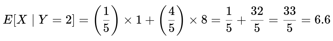
Hence, the final answer is 33/5, which is 6.6 in decimal form.
Interpretation and Intuition
The result shows that if we already know a “4” happens exactly on the second roll, it slightly constrains the possible outcomes of the first roll. There is a 1/5 chance that the first roll was “1.” If that occurs, we are done at roll 1 for X. Otherwise, we begin effectively a new “search” for “1” starting from roll 3, leading to an expected total of 8 rolls to see the first “1” in that scenario. The weighted average of these yields 6.6.
Potential Pitfalls in Reasoning
One subtle pitfall is assuming that because the second roll is “4,” the first roll being “1” might be “impossible” or have a different probability weighting. It is not impossible; the only thing we know is that the first roll is not “4.” Another pitfall is to forget that when the first roll is not “1” and not “4,” we have not yet satisfied X, so from roll 3 onward, X follows a geometric waiting time for the first “1.” It is also crucial to handle conditional probabilities properly instead of simply averaging unconditional expectations for X in different scenarios.
Alternative Approaches
One can also frame this using conditional probability expressions for X given Y = 2 and summing over all possible values of X. Another method might involve a more formal partition of events or a Markov chain approach. However, the direct scenario-based reasoning is typically simplest for a problem like this.
Practical Verification by Simulation
It can be enlightening to run a Python simulation to empirically estimate E[X | Y = 2]. Generating a large number of trials and computing the average X in those trials for which Y = 2 will typically yield a value near 6.6.
Here is an illustrative example:
import random
import statistics

def simulate_E_X_given_Y_eq_2(num_trials=10_000_000):
    # We'll store the values of X only for the cases Y=2
    x_values = []

    for _ in range(num_trials):
        rolls = []
        # Keep rolling until we see at least one "1" and also check when we get the "4"
        # But we'll do it systematically
        y = None  # the roll number when we get first 4
        x = None  # the roll number when we get first 1

        roll_count = 0
        while True:
            roll_count += 1
            outcome = random.randint(1,6)
            rolls.append(outcome)

            # Record X if first time seeing a 1
            if x is None and outcome == 1:
                x = roll_count

            # Record Y if first time seeing a 4
            if y is None and outcome == 4:
                y = roll_count

            # Once we have both X and Y, we can stop
            if x is not None and y is not None:
                break

        # Now we check if Y == 2
        if y == 2:
            x_values.append(x)

    return statistics.mean(x_values) if x_values else None

estimated_value = simulate_E_X_given_Y_eq_2()
print("Estimated E[X | Y=2]:", estimated_value)
With a large number of trials, this simulation should yield a value close to 6.6, confirming our analytical derivation.
What if the die was not fair?
In many real-world scenarios or tricky interview variations, you might be asked to compute E[X | Y=2] for a biased die. The approach would still rely on carefully enumerating the events for the first and second rolls, but the probabilities would shift. Specifically, if the probability of rolling a “4” was p4 and the probability of rolling a “1” was p1, then:
The condition Y=2 implies the second roll is “4” and the first roll is not “4.”
You would compute the probability that the first roll was “1” or some other outcome (that is neither “1” nor “4”) in proportion to their probabilities p1 or 1 - p1 - p4.
The geometric waiting time for “1” starting from the third roll would be 1/p1 in expectation, assuming each roll is i.i.d. with the same distribution.
How does the memoryless property factor into the reasoning?
The memoryless property is relevant for certain distributions like the geometric distribution. Once you know the first few rolls have not produced a “1,” the process of waiting for a “1” effectively restarts, meaning that from that point onward, the expected number of additional rolls remains 6 for a fair die. This plays into the step where we say that if the first roll was not “1” and the second roll was “4,” from roll 3 onward, we expect to wait an average of 6 more rolls for the first “1.”
Can you elaborate on the probability that the first roll is “1” given Y=2?
Given Y=2, the first roll cannot be “4.” Among the six outcomes, “4” is excluded, so the possible values for the first roll are {1, 2, 3, 5, 6}. Each of these has probability 1/6 unconditionally, but we only consider those in which the first is not “4,” and the second is “4.” The probability for (1,4) as a pair is 1/36, and the probability for (x,4) with x in {2,3,5,6} is 4/36. Summing them up gives 5/36 as the total probability for having Y=2. Thus the conditional probability that the first roll is “1,” given Y=2, is (1/36) / (5/36) = 1/5.
Why is the final result not simply 6?
One might guess that because the expected time to see a “1” is 6 unconditionally, conditioning on Y=2 might not affect X too much. However, the condition that the second roll is “4” changes the distribution of outcomes on the first roll. That changes the probability that we have already seen a “1.” This shift in distribution leads to the final answer of 6.6, which is higher than the unconditional average of 6, reflecting that we typically are “delayed” in seeing a “1” if it did not appear on the first roll.
How would you handle a more general question E[X | Y = k]?
One can generalize the same logic for E[X | Y = k] for some k ≥ 1. Condition Y=k means that the first k-1 rolls are not “4,” and the k-th roll is “4.” Among those first k-1 rolls, we look at whether a “1” might have occurred earlier. The analysis leads to partitioning cases: maybe “1” occurred among the first k-1 rolls or it did not. If it did, that sets X to whichever roll index gave the first “1.” If it did not, from roll k+1 onward, we start a geometric waiting for “1.” The overall structure remains similar but with a larger set of possible outcomes for the preceding rolls.
Could you explain the meaning of X = 1 in scenario 1 more carefully?
If the first roll is “1,” that immediately satisfies the condition “we have observed the first 1 on roll 1.” Hence X=1. Even though Y=2 indicates the second roll is the first “4,” that does not conflict with the first roll being “1.” Those events can coincide. The only conflict would be if the first roll were “4,” which cannot happen given Y=2.
Are there any edge cases if Y=2 never occurs?
In certain contrived distributions or extremely small sample simulations, it is possible you never see the event Y=2 in a finite simulation. In theory, for a fair die, the probability is always positive, so Y=2 can happen. Over enough trials, you will see many occurrences of Y=2. The only real “edge case” is if your simulation or reasoning incorrectly includes scenarios that contradict Y=2 (like the first roll being “4”) or excludes valid scenarios (like the first roll being “1”).
Final Answer
Below are additional follow-up questions


so

Thus for scenario 2:

Weight each scenario by the conditional probabilities:
• Probability(Scenario 1 | Y=2) = 1/5, • Probability(Scenario 2 | Y=2) = 4/5.
Hence:
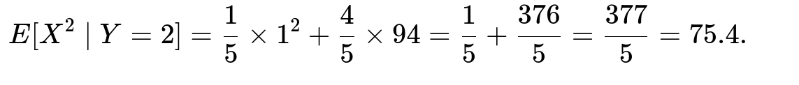
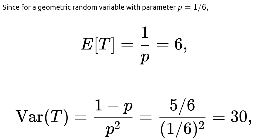
Then, if you want Var(X∣Y=2]:

Possible pitfalls: • Forgetting to square the entire expression (2+T). • Mixing up unconditional vs. conditional probabilities. • Not using the correct variance for a geometric distribution. • Overlooking that scenario 1 locks X at 1, heavily influencing the variance.
How would the reasoning change if you are told that Y=2, but you also know the actual value of the first roll?
If, in addition to knowing Y=2, you are told specifically what happened on the first roll, your distribution for X changes accordingly:
If you are told the first roll was “1,” then automatically X=1, so the conditional distribution for X collapses to that single point.
If you are told the first roll was in {2,3,5,6}, then you know you have not seen “1” in the first two rolls. Hence, from roll 3 onward, you still wait for the first “1.” That means X=2+W where W is geometric with success probability 1/6.
If you were hypothetically told the first roll was “4,” that contradicts Y=2, so that scenario is impossible.
This knowledge would drastically simplify or alter your calculation of E[X | Y=2, first roll result = r]. For instance, if r=1, X=1 exactly. If r in {2,3,5,6}, then E[X]=2+6=8.
Potential pitfalls: • Failing to see that the event “first roll = 1” can coexist with “Y=2.” • Not realizing that additional conditions typically reduce or eliminate certain scenarios. • Misapplication of the memoryless property if you are not aware which events have occurred.
If the sample size is extremely large, does the Law of Large Numbers guarantee that the observed sample mean of X given Y=2 will converge to 33/533/5 in practice?
In principle, yes. Under the assumption of identical, independent rolls, the Strong Law of Large Numbers indicates that if you run a sufficiently large number of die-roll trials and filter for those trials in which Y=2, the empirical average of X in those filtered trials should converge to the theoretical conditional expectation E[X∣Y=2]=33/5.
However, pitfalls exist: • You need a large enough sample size, not just overall but specifically for the event Y=2. The event Y=2 occurs with probability 1/6 × 5/6 = 5/36. So in a simulation or in real data, you might need tens of thousands or more total trials before you get a stable sample of that event. • If the die is not truly fair, or if the independence assumption is violated (for example, if there’s a mechanical bias or some correlation across rolls), then the observed average might deviate from the theoretical 33/5. • If you mislabel or incorrectly track which roll caused Y=2, your data would be tainted, and the average might not converge to the correct value.
How would you handle a scenario in which the die has 20 sides instead of 6?
When dealing with a 20-sided die, the same conceptual approach applies but with probability 1/20 for rolling a specific face (assuming a fair 20-sided die):
X is the number of rolls until we see a “1,” which is geometric with parameter 1/20 in the unconditional sense.
Y=2 means the second roll is the first time we see a “4.” That imposes the condition that the first roll is not “4” and the second roll is “4.”
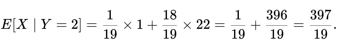
Condition Y=2 forces the first roll into any of the remaining 19 faces. Then we look at the chance that it might be “1” or some other number. Specifically: • Probability(first roll is “1” | Y=2) = 1/19. • Probability(first roll is neither “1” nor “4” | Y=2) = 17/19.
From there, the memoryless property for the event “1” reappears starting at roll 3 if the first roll was neither “1” nor “4.” You’d adjust the computations:
• Scenario 1: X=1 if the first roll is “1.” • Scenario 2: If the first roll was in {2,3,5,6,…,20} excluding “4,” we wait from roll 3 onward. The expected time from that point to see a “1” is 20 if it’s fair. So E[X]E[X] for that scenario would be 2 + 20 = 22.
Weighting:

Pitfalls: • Forgetting to exclude “4” from the set of possible first rolls under Y=2. • Mixing up the probabilities (they become 1/19 for each valid face on roll 1). • Not recognizing that the distribution to see a “1” from roll 3 onward is geometric(1/20), so the expected waiting time is 20 additional rolls from that point.
How does the calculation change if the die is fair, but we are asked for P(X<Y) or E[min(X,Y)]?
While this question shifts away from E[X∣Y=2], it still touches on subtle interactions between X and Y:
P(X<Y) is the probability that we roll a “1” before we roll a “4.” Both X and Y follow geometric(1/6) individually, but they are not independent. One approach: on each roll, you either get a “1,” a “4,” or neither. The first time you see either “1” or “4,” whichever appears first determines which is smaller. Because the die is fair, the probability we see a “1” before a “4” is 1/2. More formally, you can see that on each roll, the chance to see “1” is 1/6, the chance to see “4” is 1/6, so it’s symmetrical.
E[min(X,Y)] is the expected number of rolls to see either “1” or “4.” The probability of success (i.e., seeing either “1” or “4”) on each roll is 2/6 = 1/3, so the waiting time for “1 or 4” is geometric(1/3) with expected value 3.
Pitfalls: • Overthinking the problem and not using the fact that “1” or “4” are symmetric events if the die is fair. • Trying to treat X and Y as if they were independent. They’re not independent, but these particular questions use memoryless properties in a simpler way that can often be reasoned about directly on each roll. • Confusing P(X<Y) with P(X≤Y)—a subtle difference if both “1” and “4” appear on the same roll is actually an impossibility for a single die (you can’t get “1” and “4” simultaneously).
What if the die is fair, but we stop rolling if we reach 10 rolls without a “1” or a “4”? How does that truncation affect E[X∣Y=2]?
If there is a cap at 10 rolls (or any finite number n), meaning we stop rolling no matter what if we haven’t seen either “1” or “4,” then X and Y become truncated random variables. Their distributions no longer have infinite support:
• X can never exceed 10 if we stop at 10. • Y=2 is still the event that the second roll is the first “4,” but we also have a termination condition if we don’t see “4” up to the 10th roll.
Conditional on Y=2, you know the second roll is “4,” which means we definitely have not stopped or truncated before the second roll. So that part remains unaffected for the first two rolls. But the presence of a maximum of 10 rolls means that if you do not see a “1” by roll 10 (and you’re still rolling), you end up with X>10 or effectively X=∞ if you define it that way. In practice, you might define X to be 11 as an indicator that it was never seen in the first 10 rolls.
Hence: • Scenario 1 (first roll is “1”): X=1.. • Scenario 2 (first roll is in {2,3,5,6}, second roll is “4”): from roll 3 onward, you have a maximum of 8 more rolls to see a “1.” If you do see it, that sets X. If you do not, then X=11 as a sentinel value.
Calculating E[X∣Y=2] now would involve the probability that “1” emerges by roll 10 under that scenario, multiplied by the respective roll index, plus the probability that “1” never appears (in which case you might define X=11). The weighting would be the same approach—scenario-based with a truncated geometric distribution.
Pitfalls: • Failing to track the absorbing or stopping condition that changes the distribution tail. • Not properly accounting for the possibility that “1” might not appear at all before the cap, leading to an artificially low or incomplete expectation. • Defining X incorrectly when you don’t see “1” by roll 10. Some might define X=∞, or X=10, or X=11; the choice can alter the final numeric result.
Does the solution generalize to any pair of faces (not just 1 and 4)? For example, if X is the time until “a” appears and Y is the time until “b” appears, do we get a similar pattern?
Yes, for a fair six-sided die, if we pick any distinct faces a and b, the time to get a for the first time is geometric(1/6), and the time to get b is also geometric(1/6). The event Y=2 (the second roll is the first time we get b) means:
• The first roll is not b. • The second roll is b.
So the logic is identical, because the probability for rolling face a or face b is symmetrical as 1/6 each. If the question were E[X∣Y=2] for any distinct faces a and b, you would end up with the same numeric solution, 33/5, just interpreting “a” in place of “1” and “b” in place of “4.”
Pitfalls: • Failing to realize that for a fair die, any particular face is equally likely, so the numeric result does not depend on which faces we label “1” or “4.” • If the die is not fair, the pattern still holds conceptually, but you must update the probabilities for each face. The final numeric answer will differ.
What complications might arise if the die rolls were not independent? For instance, if there’s a Markovian dependence across rolls?
When rolls are not independent, we lose the clean geometric structure of “the time to first success.” The distribution for X or Y can be complicated by correlation between successive outcomes:
• For instance, if you have a Markov chain such that if you just rolled a 1, the next roll is less likely to be a 1, or if you just rolled a 4, maybe it’s more likely to stay at 4, etc. • The memoryless property that the geometric distribution relies upon is violated.
Hence, to compute E[X∣Y=2] you would need to carefully model how the transition probabilities in this Markov chain define the probability that the second roll is “4,” the first roll is or isn’t “1,” and how the process evolves from roll 3 onward. You could attempt:
Analytical approach: Construct the Markov chain’s transition matrix and define states that capture the event “have we seen 1 yet?” and “have we seen 4 yet?”
Simulation approach: Repeatedly simulate the chain to approximate E[X∣Y=2].
Pitfalls: • Trying to force the old geometric approach in a scenario with correlated rolls. That would lead to incorrect assumptions about distribution and expectation. • Overlooking how a Markov chain might have strongly different probabilities for transitions to “1” or “4” in subsequent rolls. • Conflating the standard fair-die independence with a system that only “looks” like a die but actually is memoryful.
How would you modify or confirm your derivation if you observed real dice behavior that suggests the side “1” is more frequent than “4”? For example, if from data you suspect the die is weighted?
In a weighted scenario, the chance of rolling a “1” might be p1, the chance of rolling a “4” might be p4, etc., summing to 1 over all six faces. Then:
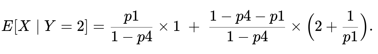
• The unconditional distribution for X is a geometric random variable with parameter p1. • The unconditional distribution for Y is a geometric random variable with parameter p4. • Condition Y=2 means the first roll is not “4” (with probability 1−p4) and the second roll is “4” (with probability p4).
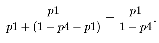
Under that condition, if the first roll is “1,” then X=1. If the first roll is in {2,3,5,6} (whatever set that sums up to 1−p4−p1 if we exclude the “4” face), from roll 3 onward, X again follows a geometric(p1). So the same scenario partition:
Probability that first roll is “1,” given Y=2, is


Hence:
Pitfalls: • Confusing the unconditional probabilities with the conditional ones. • Failing to renormalize by 1−p4 for the event that Y=2 means the first roll definitely isn’t “4.” • Using the unconditional distribution for T incorrectly (some might incorrectly scale it by the unconditional probability instead of the conditional one).