
ML Interview Q Series: Conditional Probability: Likelihood of Two Heads Given Different Head Conditions.

Browse all the Probability Interview Questions here.
A fair coin is flipped twice. Determine which event has a greater probability: obtaining two heads given that at least one flip resulted in heads, or obtaining two heads given that the second flip was heads. Then decide if this outcome changes when the coin is not fair.
Short Compact solution
Define event A as “the first toss is heads” and event B as “the second toss is heads.” For a fair coin, each of A and B has probability 1/2, and the probability that both A and B occur is 1/4. Consider two scenarios:
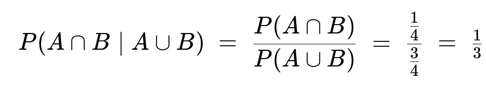
Given that at least one toss is heads, we compute the probability that both tosses are heads as

Hence, the second scenario has the larger probability (1/2 vs. 1/3). If the coin is not fair, the same conclusion holds because the probability that at least one toss is heads exceeds the probability that the second toss is heads, making the ratio for the “at least one head” case smaller than for the “second toss is heads” case.
Comprehensive Explanation
Overview of the Two Scenarios
The puzzle revolves around conditional probability. We want to know which of the two scenarios yields a higher chance of getting two heads:
Scenario (a): We are informed that at least one of the two tosses is heads.
Scenario (b): We are informed specifically that the second toss is heads.
For scenario (a), the condition changes the sample space to all outcomes that have at least one head. For scenario (b), the sample space is restricted to outcomes where the second toss is heads.
Detailed Breakdown for a Fair Coin
When the coin is fair, each toss has a 1/2 chance of landing heads (H) and 1/2 chance of landing tails (T). The possible outcomes for two tosses are HH, HT, TH, and TT, each with probability 1/4.
Scenario (a): At Least One Head
The outcomes that satisfy “at least one head” are HH, HT, and TH. Each has probability 1/4, so together they have a total probability of 3/4. Within this reduced sample space (HH, HT, TH), only one outcome (HH) achieves “two heads.” Therefore,

Scenario (b): Second Toss Is Heads
The outcomes that satisfy “second toss is heads” are HH and TH, each with probability 1/4. These two outcomes together have a total probability of 1/2. Within this sample space (HH, TH), there is only one outcome (HH) that has two heads. Therefore,

Comparing 1/3 and 1/2, we see that it is more likely to get two heads when we are told the second toss is heads, rather than being told that at least one toss is heads.
Impact of an Unfair Coin
Suppose the coin has a probability p of showing heads (and 1-p for tails). Then:
The probability of A (first toss heads) is p.
The probability of B (second toss heads) is p.
The probability of A ∩ B (both heads) is p².
The probability of A ∪ B (at least one head) is 1 - (1 - p)² = 1 - (1 - 2p + p²) = 2p - p².
We can check the two scenarios:

ParseError: KaTeX parse error: Can't use function '$' in math mode at position 71: …p \iff p \le 1,$̲$ which is gene…
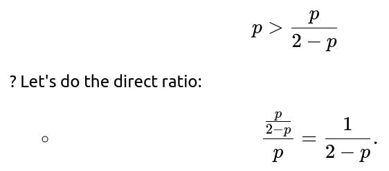
Indeed, for any valid p < 1, we have

Since (2 - p > 1) for (0 < p < 1), we have (\frac{1}{2 - p} < 1.) Hence (\frac{p}{2 - p} < p). This shows (p) is indeed larger than (\frac{p}{2 - p}) for a valid range of p (0 < p < 1). Therefore (P(A \cap B \mid B)) (which is (p)) is typically higher than (P(A \cap B \mid A \cup B)) (which is (\frac{p}{2 - p})) as long as (p) is neither 0 nor 1. Thus the result (the second scenario is more likely) still holds for an unfair coin.


This confirms that whenever you know the second toss is heads, it provides more specific information than simply knowing there is at least one head in either toss. Therefore the probability of having two heads in scenario (b) exceeds that of scenario (a), for any valid bias 0 < p < 1.
Intuitive Reasoning
In scenario (a), “at least one head” only rules out the TT outcome. But that still leaves two other single-head outcomes (HT, TH) that take away probability mass from the all-heads outcome (HH).
In scenario (b), “the second toss is heads” eliminates both T? endings (TH remains, but TT is fully excluded). This narrower condition places a heavier weight on HH as a fraction of the allowed possibilities, raising the probability of double heads.
Simulation Example in Python
It can be instructive to verify these results with a simple simulation. Below is a quick Python snippet that demonstrates the frequencies for both scenarios for a fair coin:
py import random
N = 10_000_000 count_at_least_one = 0 count_at_least_one_and_both = 0 count_second_is_heads = 0 count_second_is_heads_and_both = 0
for _ in range(N): # Each flip is either 0 for Tails or 1 for Heads first = random.randint(0, 1) second = random.randint(0, 1)
# Scenario (a)
if first == 1 or second == 1:
    count_at_least_one += 1
    if first == 1 and second == 1:
        count_at_least_one_and_both += 1

# Scenario (b)
if second == 1:
    count_second_is_heads += 1
    if first == 1 and second == 1:
        count_second_is_heads_and_both += 1
prob_a = count_at_least_one_and_both / count_at_least_one prob_b = count_second_is_heads_and_both / count_second_is_heads
print("Prob(two heads | at least one head):", prob_a) print("Prob(two heads | second toss is heads):", prob_b)
You should see that the simulated values for “two heads given at least one head” approach about 0.333..., and the “two heads given the second toss is heads” approach about 0.5.
Possible Follow-Up Questions
Why does specifying which toss is heads make a difference?
Because specifying that the second toss is heads removes more of the uncertainty: you specifically know the outcome of one particular toss. When only told that at least one of the tosses is heads, there are multiple ways this can happen (the head might be on the first toss, or the second, or both), and this dilutes the conditional probability of both being heads.
What happens if the coin is extremely biased?
Could the problem statement change if we only know “there is at least one head” but not which toss it appeared on?
This is precisely scenario (a). The fundamental difference is whether we are told that a specific toss is heads or simply that one of them is heads in an unspecified position. The puzzle is a smaller-scale version of typical conditional probability paradoxes (such as the “two children problem”), where specifying which child (or which toss) meets a condition can drastically alter the probability distribution.
How would the result change if we extended this to multiple tosses?
If we had more tosses, the difference between “knowing at least one toss is heads” and “knowing a specific toss is heads” can grow more pronounced. For instance, if you have 3 or more tosses, being told “at least one is heads” excludes only the case of all tails, whereas learning that “the nth toss is heads” excludes all sequences in which the nth toss is tails, narrowing the possibilities more significantly for the event of all heads.
Does the Bayesian formula help clarify these calculations?
Yes. The crux is to view


This straightforward application of Bayes’s rule is the mathematical basis for all the reasoning above.
How can we ensure no mistakes when applying these ideas in real-world problems?
Common pitfalls include:
Mixing up the event of “at least one is heads” with “exactly one is heads.”
Failing to explicitly write out the sample space after applying the condition.
Forgetting that specifying which toss is heads is more restrictive than not specifying the toss.
In practice, carefully enumerating the possible outcomes that satisfy a condition helps avoid mistakes, especially for more complex scenarios involving multiple events or partial information.
Below are additional follow-up questions
What if the problem is extended to three coin tosses?
One might wonder how the logic changes if, instead of two tosses, there are three tosses and we are given certain partial information (like "at least one toss showed heads" or "the third toss was heads"). How does the reasoning evolve in that scenario?
When dealing with three tosses, it is essential to carefully account for all possible outcomes and their probabilities. For a fair coin, the sample space of three tosses is composed of eight equally likely outcomes: HHH, HHT, HTH, THH, HTT, THT, TTH, and TTT. If we are told that at least one toss is a head, we exclude TTT, leaving seven possible outcomes. If we want the probability that all three are heads (HHH) given that at least one is heads, we then consider:
The total number of valid outcomes: 7.
The favorable outcome (HHH) is just 1.
So, under the event “at least one head,” the probability of three heads would be 1/7.
By contrast, if we are given the event that “the third toss was heads,” we filter out all outcomes where the third toss is T. That leaves the four outcomes: HHH, HTH, THH, TTH — but the last one (TTH) ends with H only if the third toss is H, so we have HHH, HTH, THH, and TTH. Now, the probability of HHH (three heads) given the third toss was heads is 1 out of these 4 valid outcomes, which is 1/4. This shows that specifying which particular toss is heads (the third toss, for instance) typically yields a different conditional probability than the vague statement “at least one toss is heads,” similar to the two-toss scenario but extended to three tosses.
A frequent pitfall is to forget to systematically enumerate all valid outcomes after a condition is imposed. Another subtlety is if the problem states something like “the third toss showed heads when observed,” and we do not know about the first or second toss. In real-world scenarios, especially with an actual physical experiment, there could be measurement errors or ambiguous observations that further complicate the analysis.
How does this probability puzzle connect to Bayesian updating in real-world applications?
In real-world settings, we often face scenarios where we gain partial information about the outcomes of uncertain events (e.g., sensor data in a robotics task, partial test results in a medical diagnosis, or partial logs in software). Each piece of information changes our belief about the underlying true state. We use Bayesian updating to incorporate new evidence.
In the coin-toss problem, when we learn that “at least one toss was heads,” or that “the second toss was heads,” we effectively apply a Bayesian update. Our prior probability distribution over all possible toss outcomes is modified by the newly observed evidence. Concretely:
The prior is the probability distribution before any evidence (all outcomes are equally likely for a fair coin).
The likelihood of the evidence given each outcome is how probable it is that we would see “at least one head” or “a specific toss is heads” if that outcome were indeed true.
The posterior distribution is then computed proportionally to the product of the prior and the likelihood.
A potential pitfall is ignoring the prior entirely or mixing up the direction of inference (confusing P(A|B) with P(B|A)). In machine learning applications, a similar issue arises if we incorrectly update model parameters or if we conflate the probability of data given the model with the probability of the model given the data.
How do these conditional probabilities change if the coin has a prior chance of landing heads that is unknown and must be estimated?
If we do not know the fairness of the coin beforehand, we might place a prior distribution over the bias parameter p (the probability of landing heads). For instance, a Beta distribution (commonly Beta(1,1) if we start with no assumptions) is a standard conjugate prior for the Bernoulli process.
In that case, each observation of heads or tails updates the parameters of the Beta distribution. For example, if we start with Beta(1,1) and observe one head, one tail, the posterior becomes Beta(2,2). Then, when asked about the probability of seeing two heads in future coin tosses, we would integrate over the posterior distribution of p:
The same logic applies if we are told “at least one toss is heads,” in which case our updated distribution might exclude certain outcomes or weight them differently. Pitfalls here include forgetting to marginalize over the uncertainty in p or incorrectly applying the Beta-Bernoulli updating formula. Realistically, in a live setting (like online A/B testing), ignoring these posterior updates leads to an overconfident or underconfident model of the coin's bias.
Below is a more detailed, step-by-step explanation of how we handle an unknown coin bias using a Beta prior and Bayesian updating:
Interpreting the Unknown Bias of the Coin
When we say “the coin might be unfair, and we do not know its bias,” we mean we do not know the true probability (p) of landing heads. Instead of assuming (p = 0.5), we treat (p) itself as a random variable. Our goal is to update our belief about (p) based on the observed tosses.
Using a Beta Prior
We choose a Beta distribution as a prior over (p). A Beta distribution is often written as:
where (\alpha) and (\beta) are positive parameters that shape the distribution. For the special case (\alpha = 1, \beta = 1), the Beta distribution is uniform on the interval ([0,1]). This corresponds to having no initial preference for any particular bias—every value of (p) is equally likely.
Why the Beta Distribution Is Useful
The Beta distribution is the conjugate prior for the Bernoulli (coin-toss) process. This means if the prior on (p) is Beta((\alpha, \beta)), and we observe heads or tails, then the posterior distribution (our updated belief about (p)) remains in the Beta family but with updated parameters.
If you see 1 head, you increase (\alpha) by 1.
If you see 1 tail, you increase (\beta) by 1.
Hence, if we start with (\text{Beta}(1,1)) (the uniform prior) and observe 1 head, 1 tail, the posterior becomes:

The Posterior Distribution
In general, if the prior is (\text{Beta}(\alpha, \beta)) and we observe (h) heads and (t) tails, then the posterior for (p) will be:

Each additional head increments (\alpha); each additional tail increments (\beta).
Predicting Future Tosses
Suppose after seeing some heads and tails, your posterior is (\text{Beta}(\alpha, \beta)). Now you want to know, for instance, the probability that the next toss is heads. Under the posterior distribution, this probability is:

(This is the mean of the Beta((\alpha, \beta)) distribution.)
Probability of Two Heads in Two Future Tosses
If you want the probability of observing two heads in two future tosses, you cannot simply say (\left(\frac{\alpha}{\alpha + \beta}\right)^2). Instead, you account for the fact that (p) itself is unknown and described by (\text{Beta}(\alpha,\beta)). Formally, you compute:

This integral reflects the average of (p^2) weighted by how likely each (p) value is under the Beta((\alpha,\beta)) distribution. One can solve this integral analytically or use known Beta function identities:

This formula is a more precise measure because it integrates over all possible biases (p), rather than just plugging in a single point estimate.
For instance, if (\alpha=2,;\beta=2) (the posterior after observing one head and one tail with a (\text{Beta}(1,1)) prior), then:
So, if you have (\text{Beta}(2,2)) as your posterior, the probability of seeing two heads in two new tosses is (0.30) (i.e., 30%).
Adapting to Conditional Events
If you are told “at least one toss is heads” or “the second toss is heads,” this observation also updates your distribution of (p). In principle, you might do:
Identify the likelihood of that observation under each possible value of (p).
Multiply the prior by that likelihood to get the unnormalized posterior.
Normalize to ensure the posterior integrates to 1.
In more complicated scenarios (e.g., multiple coin tosses or partial observations), you may have to carefully enumerate which sequences of heads/tails are consistent with “at least one head” or “second toss is heads” and update accordingly.
Pitfalls and Subtleties
Incorrectly ignoring uncertainty in (p): A common mistake is to just replace (p) with a single point estimate (e.g., sample mean (\hat{p})) and ignore the uncertainty. Proper Bayesian analysis integrates over all possible values of (p).
Forgetting the Prior Influence: Even if you see zero heads in two tosses, your posterior is not (\text{Beta}(1,3)) with mean (1/4) by accident; it’s because the Beta(1,1) plus the two tails updates (\beta) from 1 to 3. The prior ensures that even if you see only tails, you still have a nonzero probability for heads in future tosses.
Over/Under Confidence: If the prior is too strong (large (\alpha+\beta)), new evidence of heads or tails won’t shift your posterior much. If the prior is too weak, your posterior might swing drastically with a small number of tosses.
Computational Aspects: In real-world scenarios (e.g., online A/B testing), we update (\alpha) and (\beta) often. Make sure to keep track of them without floating-point overflow or rounding issues, especially if you accumulate many observations.
Interpreting “At Least One Head” Condition: If you do not explicitly incorporate that condition into your Bayesian update, you might incorrectly weight certain outcomes. Proper enumeration or usage of the law of total probability is important.
Small Python Example
Below is a brief Python snippet showing how to compute the integral numerically (though in practice you might just use the closed-form formula). We’ll assume we have (\alpha=2, \beta=2) as our posterior:
import numpy as np
from scipy.stats import beta

alpha, beta_param = 2, 2

# Probability of two heads in two future tosses, computed by sampling
num_samples = 10_000_00
samples = np.random.beta(alpha, beta_param, size=num_samples)
# Probability in each sample that we get 2 heads in 2 tosses ~ p^2
prob_estimate = np.mean(samples ** 2)

print("Estimated Probability of 2 heads in 2 tosses:", prob_estimate)

# Compare with the known analytical solution:
# alpha*(alpha+1) / [(alpha+beta)*(alpha+beta+1)] = 2*3 / [4*5] = 6/20 = 0.3
This code samples many candidate values of (p) from the Beta((\alpha,\beta)) distribution, then for each sample calculates (p^2). Averaging those results approximates the integral. The analytical formula for Beta(2,2) is exactly (0.30).
In summary, the key idea is that when the coin’s bias (p) is unknown, we maintain a probability distribution over (p). Each head or tail observation updates that distribution via simple rules if we use a Beta prior. Then, any forecast about future heads or tails involves averaging over that updated distribution rather than treating (p) as a known constant.
In practical terms, how do you address situations where partial observation might be biased?
Sometimes, the statement “we observed that the second toss was heads” might come from a biased sampling process. Perhaps the coin toss is recorded only if it is heads, and you never record tails (or the observation device malfunctions in a systematic way). This leads to selection bias: the condition that “the second toss was heads” does not just condition on a real neutral observation but might be more likely to appear in the data if there's a skewed mechanism that favors observing heads.
From a machine learning perspective, a prime example is a dataset with sampling bias. We might only have examples of positive outcomes (e.g., success cases) because negative outcomes were either not recorded or downsampled. The immediate pitfall is applying standard probability or machine learning algorithms that assume random sampling of data, which can produce erroneous estimates of outcomes and lead to miscalibrated probabilities.
A robust approach is to model the observation process itself. For instance, if we suspect that heads results are over-represented by a factor of 2, we incorporate that information into our likelihood model or weighting scheme. In real applications like fraud detection or medical diagnostics, failing to model the observation bias can lead to systematically incorrect inferences about true event rates.
What happens if the statement changes to “At least one toss came up heads on a specific day” rather than “At least one toss came up heads” in general?
Subtle changes in language that specify “on a particular day” (or a particular instance) can alter which sample space we consider. For instance, if we say “at least one toss was heads on Tuesday,” we might be implicitly specifying that we’re only considering sets of tosses that happened on Tuesday and ignoring anything else. Or if there is some information about how many times the coin was tossed on different days, it can change the underlying probabilities.
A subtle pitfall is incorrectly ignoring or double counting the date/time context. In simpler terms, if you toss a coin multiple times across multiple days, the prior day’s outcomes may or may not be relevant to the statement “today’s toss had at least one head.” If the events are truly independent day-to-day, it might have no bearing, but if the day correlates with the coin's environment (e.g., temperature could affect the coin’s rotation in some minuscule way), it becomes a different set of conditional probabilities.
In real-world data science tasks, context is paramount. For example, if a user action (like clicking on an ad) is known to happen “at least once on a weekend,” analyzing that event must incorporate how user behavior changes on weekends compared to weekdays. Ignoring that subtlety could lead to flawed user behavior models.
How would you explain to a beginner why the probability “at least one toss was heads” leads to a different result than “the second toss was heads,” even though both statements describe only one head?
The main confusion for beginners often arises from the fact that “at least one toss was heads” includes multiple possible outcomes (like HT, TH, HH in the two-coin scenario), while “the second toss was heads” focuses on only half of the sample space (HH or TH) but in a very specific manner. Although both statements reveal the presence of a head, they are not equivalent pieces of evidence. One lumps many outcomes (including the possibility of more than one head), while the other zooms in on exactly which toss produced that head.
A common pitfall is to conflate the notion that “heads was seen” with “exactly one head was seen in a specific position.” When working through probabilities, beginners should be taught to enumerate outcomes and their probabilities carefully. For a fair coin with two tosses, “the second toss was heads” cleanly slices the sample space into two sets (second toss heads vs. second toss tails). But “at least one head” slices the sample space in a different, often larger set. Each slice changes the relative proportions of outcomes that fit within that slice, leading to different conditional probabilities.
In practical terms, explaining this in an intuitive story-based way (like physically listing the possible sequences or drawing a decision tree) often helps. Additionally, it’s essential to reiterate that the event “at least one head” doesn’t give you any clue as to which toss is the head—there are multiple equally valid ways for that event to happen—whereas “the second toss was heads” removes ambiguity about which toss delivered the head.
Could these ideas be applied to anomaly detection where at least one measurement is flagged as abnormal?
Yes. In anomaly detection for systems that generate multiple measurements (for instance, multiple sensors on a machine), one might receive partial alerts such as “at least one sensor flagged an anomaly.” This is analogous to “at least one coin toss was heads.” Determining the likelihood of a genuine system fault under that condition requires enumerating or modeling all possible ways the sensors can flag anomalies. If you identify exactly which sensor flagged an anomaly (similar to specifying which toss came up heads), that is more specific information and changes the probabilities of true failure modes.
A pitfall is ignoring correlation among sensors. If you assume each sensor is an independent coin toss, you might underestimate or overestimate the overall anomaly probability when the sensors actually share dependencies (like environmental noise that affects them all simultaneously). In real-world systems (e.g., manufacturing lines, data center hardware), sensor readings can be correlated. If we only know “at least one sensor triggered,” we need to incorporate the possibility that correlated triggers could occur more frequently than independent triggers would.
Another subtlety is that certain sensors might have different false positive/negative rates. If the “second sensor always flags anomalies more reliably,” it is parallel to having a coin with an uneven probability of heads. Correctly adjusting for those different detection rates is crucial to accurately compute the probability of a real anomaly, conditioned on the partial observation that some sensor or a particular sensor has flagged an issue.