
ML Interview Q Series: Conditional Battery Survival Probability Using Exponential Mixture Models.

Browse all the Probability Interview Questions here.
A battery comes from supplier 1 with probability p1 and from supplier 2 with probability p2, where p1 + p2 = 1. A battery from supplier i has an exponentially distributed lifetime with expected value 1/mu_i for i=1,2. The battery has already lasted s time units. What is the probability that the battery will last for another t time units?
Short Compact solution
First, the distribution for X (the battery lifetime) is given by mixing two exponential distributions:

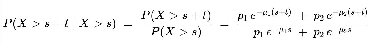
Then, using the definition of conditional probability,
Comprehensive Explanation
Overview of the Problem
We have a random variable X representing the lifetime of a battery. There are two suppliers:
Supplier 1 provides a battery with probability p1
Supplier 2 provides a battery with probability p2
where p1 + p2 = 1.
A battery from supplier i has an exponential lifetime distribution with rate parameter mu_i (i=1,2). This means that the lifetime T of that battery from supplier i satisfies:
T ~ Exponential(mu_i)
The expected lifetime is 1/mu_i.
Hence, the overall lifetime X is a mixture of two exponential distributions.
Mixture Distribution
Since the battery is chosen from supplier 1 or supplier 2 randomly (with probabilities p1 and p2), the survival function for the random variable X is:
P(X > x) = p1 * e^(-mu1 x) + p2 * e^(-mu2 x)
for x >= 0. This arises from the law of total probability, applying:
P(X > x) = P(X > x | A1)*P(A1) + P(X > x | A2)*P(A2) = e^(-mu1 x)*p1 + e^(-mu2 x)*p2.
Conditional Probability Calculation
We want to find the probability that the battery lasts an additional t time units, given that it has already survived s time units. Symbolically:
P(X > s + t | X > s).
By definition of conditional probability:
P(X > s + t | X > s) = P(X > s + t) / P(X > s).
We already know:
P(X > s) = p1 * e^(-mu1 s) + p2 * e^(-mu2 s).
Similarly,
P(X > s + t) = p1 * e^(-mu1 (s + t)) + p2 * e^(-mu2 (s + t)).
Hence, the desired conditional probability is:
[ p1 e^(-mu1 (s + t)) + p2 e^(-mu2 (s + t)) ] / [ p1 e^(-mu1 s) + p2 e^(-mu2 s) ].
Why This Expression Differs From the Pure Exponential Memoryless Formula
A single exponential distribution has the memoryless property: for an exponential random variable Y with rate mu, we get:
P(Y > s + t | Y > s) = e^(-mu t).
However, when X is a mixture of two exponentials, that mixture no longer possesses the pure memoryless property. Because we do not know from which supplier the battery came once we observe a partial lifetime s, the updated (posterior) mixture weights can shift. Thus, we do not simply get e^(-mu t); instead, we get the ratio of two mixed exponentials at s+t and s.
Detailed Parameter Explanation
p1 and p2 (p1 + p2 = 1) are the mixing probabilities for supplier 1 and supplier 2.
mu1, mu2 > 0 are the rate parameters for each supplier's battery lifetime distribution. Larger mu_i implies a shorter expected lifetime 1/mu_i.
s >= 0 is the time the battery has already survived.
t >= 0 is the additional survival time we are asking about.
Putting it all together, if we did not know anything about which supplier the battery came from initially, we treat the overall distribution as a mixture. Upon observing survival up to time s, the posterior distribution that the battery was from supplier 1 (or 2) gets updated implicitly, which leads to the final conditional probability expression above.
Possible Follow-up Questions
1) What if mu1 = mu2 = mu?
If mu1 = mu2 = mu, then both suppliers' batteries share the same exponential distribution. In that special case, the mixture distribution essentially collapses to a single exponential with rate mu, and the distribution is truly memoryless. Then:
P(X > s + t | X > s) = e^(-mu t).
The mixture ratio remains the same at all times because there is effectively no difference between the two supplier distributions.
2) How do we compute the posterior probability that the battery is from supplier 1 given it survived s units?
We can use Bayes’ theorem. Specifically,
Posterior( from supplier 1 | survived s ) = [ p1 * e^(-mu1 s ) ] / [ p1 * e^(-mu1 s ) + p2 * e^(-mu2 s ) ].
This probability may shift from the original p1, p2 ratio depending on which exponential rate is larger. If a slower decay rate (smaller mu) is more likely to survive longer, it will dominate the posterior.
3) How can we implement a simulation to check this probability numerically?
A simple Python approach is:
import numpy as np

def simulate_mixture_exponential(p1, mu1, mu2, s, t, num_samples=10_000_000):
    # Generate which supplier each battery comes from
    supplier_flags = np.random.rand(num_samples) < p1  # True if from supplier 1
    # Generate lifetimes
    lifetimes = np.where(supplier_flags,
                         np.random.exponential(1/mu1, size=num_samples),
                         np.random.exponential(1/mu2, size=num_samples))

    # Filter those that survive at least s
    survived_mask = lifetimes > s
    survived_lifetimes = lifetimes[survived_mask]

    # Among those that survived s, check fraction that survive beyond s + t
    survived_t_mask = survived_lifetimes > (s + t)
    return np.mean(survived_t_mask)

# Example usage
p1 = 0.6
mu1 = 1.0
mu2 = 2.0
s = 5.0
t = 3.0

estimated_prob = simulate_mixture_exponential(p1, mu1, mu2, s, t)
print("Estimated P(X > s + t | X > s):", estimated_prob)
We generate random samples of lifetimes according to the mixture distribution, check how many survive s, then among those, see how many survive an additional t. This verifies the analytical result.
4) How does this concept help in real-world scenarios?
In many real-world situations, components can come from different manufacturing processes (each with a distinct failure rate). When analyzing failure times, it is vital to recognize that an overall population might be a mixture of different subpopulations. In such scenarios, ignoring the mixture aspect and assuming a single exponential can lead to incorrect conclusions about remaining lifetimes or reliability. Identifying the mixture probabilities and the different rates allows for more accurate modeling, reliability estimates, and maintenance schedules.
5) What happens if s or t are zero or negative?
Typically, s and t should be non-negative because they represent elapsed times or additional times. If s=0, then the probability P(X > t | X > 0) is simply P(X > t)/P(X > 0) = P(X > t) because P(X > 0) = 1. If t=0, then P(X > s + 0 | X > s) = 1. Negative values do not make sense in this context because the exponential distribution domain is nonnegative.
6) Are there any edge conditions that cause numerical instability in implementation?
If mu1 or mu2 is extremely large, then e^(-mu_i x) can underflow for moderate to large x.
If s or t are very large, direct computation of e^(-mu_i (s + t)) might underflow to zero on a computer. One typical remedy is to factor out a common term from the numerator and denominator exponentials, or to use log-sum-exp numerical techniques for stability.
All of these subtle points can arise in practical code. It is important to handle floating-point underflow or overflow carefully, especially when s or t is large.
Below are additional follow-up questions
1) If we only have partial data on lifetimes (some are censored), how would we estimate p1, mu1, and mu2?
One of the practical challenges in real-world reliability studies is that some components may still be functioning at the time you collect the data, so their exact failure time is unknown (right-censored). Or you might only know that a certain fraction failed within an interval. In such scenarios, the maximum likelihood estimation (MLE) procedure for mixture distributions must incorporate censoring.
Key Points:
Censored data: If a component has not failed by time t_obs, you only know X > t_obs. This partial information must be included in the likelihood function appropriately.
Likelihood contribution: For any battery that failed at time x, the likelihood contribution is p1 * mu1 * exp(-mu1x) or p2 * mu2 * exp(-mu2x), each weighted by the mixing probability. For censored batteries that survived time x, the contribution is p1 * exp(-mu1x) + p2 * exp(-mu2x).
Estimation method: Numerical optimization (e.g., gradient-based or expectation-maximization for mixtures) is typically employed. The EM algorithm is well-suited to mixture models. With exponential mixture plus censoring, we set up the log-likelihood with all available data and then iterate to find MLE estimates for p1, mu1, mu2.
Potential Pitfalls and Edge Cases:
Identifiability: If the two rates mu1, mu2 are close together or if few failures are observed, it can be difficult to distinguish them. Parameter estimates may have large variance.
Initial guesses: EM or other optimization algorithms can get stuck in local optima, especially if started with poor initial guesses.
Data imbalance: If an overwhelming fraction of the batteries is from one supplier in reality, the mixture might be almost indistinguishable from a single exponential, complicating the inference of the minority supplier’s parameters.
2) What if we suspect the supplier’s lifetimes are not purely exponential?
Although it is typical to model certain lifetimes with an exponential distribution, some real-world failure processes deviate from a constant hazard rate. In such cases, an exponential assumption might be overly simplistic.
Key Points:
Possible distributions: Weibull, Gamma, or Lognormal are commonly used if the hazard rate is not constant.
Mixture of generalized distributions: Instead of mixing exponentials, you might mix two Weibull or two Gamma distributions if each supplier’s battery has that form.
Impact on memorylessness: Once we deviate from exponential for at least one supplier, we lose the memoryless property. The mixture becomes more complex, and the conditional survival function has no simple closed form.
Model selection: You can use goodness-of-fit tests or information criteria (AIC/BIC) to decide if an exponential mixture is appropriate.
Potential Pitfalls and Edge Cases:
Overfitting: Introducing more flexible distributions (like Weibull with multiple parameters) can overfit small datasets.
Complex parameter estimation: Mixtures of higher-parameter distributions typically require more advanced numerical optimization or MCMC methods for Bayesian approaches.
3) How do we handle if we discover a third (or more) suppliers?
In many manufacturing chains, it is possible that the real system is not just two suppliers but multiple sources, each with its own rate parameter.
Key Points:
Generalization: You extend from a 2-component mixture to an n-component mixture. The overall survival function becomes the weighted sum of exponentials (or other distributions).
Parameter explosion: Each additional supplier adds one more rate parameter mu_i and one more mixing probability p_i (with the constraint p1 + ... + pn = 1). This increases complexity.
Interpretation: The process for conditional probability after surviving time s remains the same conceptually: you compute the ratio of P(X > s+t) over P(X > s), but now with more terms in each sum.
Potential Pitfalls and Edge Cases:
Identifiability and data requirements: With many components in the mixture, you need substantially more data to reliably estimate the distinct parameters. Sparse data can yield very wide confidence intervals for the rates.
Numerical stability: Summations of exponentials with large negative exponents can cause underflow or overflow in floating-point arithmetic as n grows.
4) What happens if one of the rates is extremely high or extremely low?
Suppose mu1 >> mu2. That would imply one supplier’s batteries have a much smaller mean lifetime compared to the other. In a mixture distribution, this can lead to certain boundary behaviors.
Key Points:
Dominance at early times: If mu1 is much larger, then the probability of failing early for that subgroup is higher. Observing a battery survive a moderately large s might thus drastically shift the posterior probability in favor of the slower-failing supplier.
Numerical underflow: If mu1 is large and s is big, terms like exp(-mu1*s) might become extremely small. This can cause numerical issues in software implementations.
Potential Pitfalls and Edge Cases:
Degenerate mixture: If mu1 or mu2 goes to infinity, effectively p1 or p2 might become irrelevant. For instance, if mu1 is extremely large, that battery type nearly always fails quickly, so after a certain s, the probability that we have that type is negligible.
Parameter estimation instability: If data suggests one group has extremely short lifetimes and the other extremely long, it is easy for iterative optimization routines to overshoot or produce non-physical estimates.
5) Is there a simple approximation if we only care about very large s and t?
For large s (and thus s+t), exponential terms e^(-mu_i*(s + t)) can be quite small. However, one supplier’s term might dominate if mu1 < mu2 or vice versa.
Key Points:
Dominant rate: If mu1 < mu2, the battery from supplier 1 has a higher chance to live longer. Over large s, the survival function for the smaller rate will dominate in the sum. Thus, you can approximate the mixture by whichever exponential distribution is slower.
Posterior weighting: After surviving s, the updated probability that the battery belongs to the slower-failing supplier can become very close to 1 if s is large.
Potential Pitfalls and Edge Cases:
Accuracy of approximation: If the rates are not drastically different, ignoring one term may cause inaccuracies.
In-between domain: For moderate s, neither rate fully dominates. The approximation might be inaccurate if s is not large enough to effectively rule out one supplier.
6) How could we incorporate prior knowledge about the rates in a Bayesian analysis?
Sometimes we have expert knowledge or historical data about mu1, mu2, or p1 that we want to incorporate before observing any new battery lifetimes.
Key Points:
Choice of priors: Conjugate priors for exponential rates often involve Gamma distributions. For p1, p2, a Beta prior is typical.
Posterior distribution: Given observed failure times (and survival times if censored), we update these priors to posterior distributions for mu1, mu2, and p1.
Credible intervals: A Bayesian approach naturally provides credible intervals around each parameter, reflecting uncertainty. This can be especially valuable if data are limited.
Potential Pitfalls and Edge Cases:
Sensitivity to priors: With limited data, the choice of priors might heavily influence posterior estimates.
Computational complexity: If the mixture is complicated and data are large, MCMC can be computationally expensive. Variational inference or specialized sampling methods might be needed.
7) How does the hazard rate evolve over time for this mixture distribution?
For a mixture of exponentials, the hazard rate h(t) is not constant. It is given by:
h(t) = f(t) / S(t),
where f(t) is the PDF and S(t) is the survival function. Because f(t) is the derivative of S(t), each exponential term’s contribution changes over time.
Key Points:
Non-monotonic hazard: Unlike a single exponential distribution (which has a constant hazard), a mixture of exponentials can have a hazard rate that decreases or increases, depending on how the weighting shifts to the slower or faster rate over time.
Behavior at early vs. late times: Early on, the faster-failing component may dominate, causing a higher hazard rate initially. As time goes on, the surviving population is more likely from the slower component, potentially lowering the hazard rate.
Potential Pitfalls and Edge Cases:
Interpreting hazard incorrectly: If an engineer assumes a constant hazard (pure exponential) for a mixture, they might under- or over-estimate the reliability at later times.
Complex shape: A two-exponential mixture can produce hazard rate curves that have peaks or inflection points, which might be unexpected if you only deal with single exponentials.
8) Could there be correlation between which supplier is chosen and how the battery is used?
In some real-world situations, the choice of supplier might be correlated with usage patterns or environmental conditions (e.g., heavier loads might consistently use supplier 1’s batteries). This complicates the simple mixture model assumption that supplier choice and usage profile are independent.
Key Points:
Conditional distribution shift: If usage environment is more stressful for one supplier’s batteries, then even if the inherent design is the same, the effective rate might differ due to different usage intensities.
Stratified modeling: A more refined approach would treat usage environment as a covariate. Instead of a simple mixture, you might build a regression-like model (e.g., survival analysis with covariates in a parametric or semi-parametric setting).
Data collection challenges: You would need to track not just the supplier but also how each battery is deployed, to isolate the effect of usage from the effect of supplier differences.
Potential Pitfalls and Edge Cases:
Ignoring confounders: Failing to account for usage differences can lead to incorrect estimates of supplier reliability.
Overly complicated model: Including too many covariates can require significantly larger data sets to produce stable estimates.