ML Interview Q Series: Confidence Intervals: Simply Explaining Uncertainty in Statistical Estimates

Browse all the Probability Interview Questions here.
How would you explain a confidence interval in everyday language to an audience without a technical background?
Short Compact solution
Imagine you want to figure out a population quantity, such as the average height of adult males in a certain country. You collect a sample of a thousand random individuals, compute the sample mean, and realize this average can shift depending on which thousand people you picked. A confidence interval is a way to capture the uncertainty around that sample mean by creating an interval with a lower and upper bound. If you were to repeat the process of sampling many times, a 95% confidence interval would contain the true average for about 95% of those repeated experiments. The narrower the interval, the more precise your estimate is, reflecting less uncertainty around that sample average.
Comprehensive Explanation
A confidence interval is a statistical concept used to indicate the reliability or uncertainty around an estimate. Suppose you want to determine the mean value of a certain parameter (such as average height or average income) in a large population. Because you cannot measure every individual in that population, you take a sample. You compute the mean of the sample, which gives you one estimate. However, if you repeatedly gathered new samples of the same size, each would yield slightly different means.
A confidence interval addresses this variability by providing a lower and upper bound around your sample mean. These bounds reflect how your estimate might shift if you sampled repeatedly, under assumptions such as normality (or large sample size by the Central Limit Theorem) and known or estimated variance. Typically, you choose a “confidence level,” often 95%, to communicate that if you were to repeat the entire sampling process a large number of times, approximately 95% of those confidence intervals would include the true population mean.
To see why this helps, consider that a single number (the sample mean) lacks any expression of uncertainty. When we attach a confidence interval to that mean, we are effectively saying, “The parameter is likely in this range, given the data we observed, and the assumptions we made.” A narrower interval implies higher precision in the estimate (less uncertainty), whereas a wider interval indicates more uncertainty or variability in the data.
In a more formal sense, for a population mean, the confidence interval is often approximated using the sample mean and sample standard deviation. If the sample size is reasonably large, the lower and upper bounds of a 95% confidence interval are found by adding and subtracting a margin of error from the sample mean. This margin of error is typically computed by multiplying a critical value (often from the normal distribution, like 1.96 for 95% confidence) by the standard error of the mean (sample standard deviation divided by the square root of the sample size).
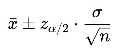
Below is a simple expression for a 95% confidence interval for the mean when the population standard deviation is unknown but the sample is large enough that the normal approximation is reasonable:


This formula indicates we take our sample mean and move a bit lower and higher by the margin of error. In practice, if the sample is smaller or if the distribution is not close to normal, more careful approaches (e.g., t-distribution, bootstrap methods) can be used to account for additional uncertainty.
Potential Follow-up Questions
How does sample size affect the width of a confidence interval?
The size of the sample has an inverse relationship with the width of the confidence interval. As you increase your sample size, the standard error of the mean (which is roughly the standard deviation of the sample divided by the square root of the sample size) becomes smaller. A smaller standard error leads to a narrower margin of error, and thus a narrower confidence interval.
Is it correct to say that there is a 95% probability the true mean is in the interval?
A subtlety with confidence intervals is that they are constructed under a frequentist interpretation of probability. The true mean is fixed, while the interval would vary if you sampled repeatedly. Strictly speaking, it is more precise to say: “If we repeated this experiment many times, approximately 95% of those confidence intervals calculated from the samples would contain the fixed (but unknown) true mean.”
Many people casually say, “There is a 95% chance the true mean lies in the interval,” but that is a Bayesian-sounding statement rather than a strictly frequentist interpretation. In everyday discussions (especially with non-technical audiences), the casual statement is often considered acceptable. However, in a technical or academic context, the correct frequentist interpretation is about repeated sampling, not probability for the fixed true mean.
What is the difference between a confidence interval and a prediction interval?
A confidence interval describes uncertainty around an estimate of a parameter (like the population mean). A prediction interval describes uncertainty around the actual observed value in a single new observation or a future data point.
Confidence interval for the mean: “We think the average is between A and B.”
Prediction interval: “We think the next observed value for an individual data point will fall between C and D.”
Prediction intervals are typically wider because they must account for both the uncertainty in the mean and the inherent variability of individual observations.
How can you make a confidence interval narrower without reducing the confidence level?
There are several approaches:
Increase sample size: As n grows, the standard error decreases, reducing the margin of error.
Use a method that decreases variability: For instance, reduce measurement noise or collect more consistent data.
Adopt a more refined sampling strategy: Techniques like stratified sampling can reduce variability in estimates, leading to a narrower interval.
However, for the same dataset and the same method of estimating the parameter, narrowing the interval typically forces you to lower your confidence level (e.g., going from 95% to 90%). To keep the same confidence level but get a narrower interval, you generally need more or better-quality data.
How do you construct a confidence interval programmatically in Python?
Below is an example using basic Python libraries and the normal approximation for a sample mean when n is large. Suppose we have some data in a list called data:
import numpy as np
from scipy import stats

data = [60, 61, 63, 59, 65, 62, 60, 68, 70, 58]  # Example data

# Convert to a numpy array for convenience
arr = np.array(data)

# Sample mean
x_bar = np.mean(arr)

# Sample standard deviation
s = np.std(arr, ddof=1)  # ddof=1 for sample standard deviation

# Sample size
n = len(arr)

# Confidence level
confidence_level = 0.95

# For large n, or if you assume the population standard deviation is known,
# you might use a z-value. For a smaller sample you might use the t-distribution.
# We'll illustrate the t-distribution approach:
t_critical = stats.t.ppf((1 + confidence_level) / 2, df=n-1)

# Standard error of the mean
sem = s / np.sqrt(n)

# Margin of error
margin_of_error = t_critical * sem

lower_bound = x_bar - margin_of_error
upper_bound = x_bar + margin_of_error

print("Sample Mean:", x_bar)
print(f"{int(confidence_level*100)}% Confidence Interval: ({lower_bound}, {upper_bound})")
Key points in this code example:
We compute the sample mean (
x_bar) and sample standard deviation (s).We choose a 95% confidence level (
confidence_level = 0.95).We retrieve the appropriate t-critical value from
stats.t.ppf, since we have a relatively small sample (10 points in this example).We multiply the critical value by the standard error (
sem = s / sqrt(n)) to get the margin of error.We subtract and add this margin of error from the mean to get the lower and upper bounds of our confidence interval.
What practical pitfalls should one watch out for when using confidence intervals?
Non-representative samples: If the sample is biased or unrepresentative of the population, the confidence interval might be misleading.
Incorrect distribution assumptions: For small samples or heavily skewed distributions, the common normal or t-distribution assumptions may not hold.
Multiple comparisons: If you calculate many confidence intervals for multiple parameters, you have to adjust for the fact that some intervals might be “correct” merely by chance.
Misinterpretation: As mentioned, confidence intervals do not directly state a probability that the true parameter is in the interval; they reflect the properties of repeated sampling.
Below are additional follow-up questions
How do confidence intervals differ from credible intervals in a Bayesian context?
Confidence intervals (CIs) are rooted in frequentist statistics, where the parameter being estimated is viewed as a fixed, unknown quantity, and the interval is constructed so that repeated experiments would contain the true parameter a specified percentage of the time. Credible intervals, on the other hand, come from Bayesian statistics, where the parameter itself is treated as a random variable with a prior distribution, and the observed data updates that prior to form a posterior distribution. A credible interval is derived directly from this posterior, meaning it reflects the range of parameter values that have a specified posterior probability.
From a practical standpoint, one main difference is interpretation. A 95% credible interval directly states that there is a 95% probability the parameter lies in that interval, under the chosen prior and likelihood assumptions. In contrast, a 95% confidence interval does not assign a probability to the fixed parameter; it discusses the proportion of intervals that would capture the true parameter if you repeated the experiment infinitely many times. In real-world applications, the choice between confidence intervals and credible intervals can hinge on philosophical considerations about interpreting probability and uncertainty, as well as practical factors like available computational methods and prior knowledge.
Potential pitfalls and edge cases
Choice of priors in Bayesian analysis: If priors are poorly chosen or overly influential, the credible interval might be misleading.
Misinterpretation: Many individuals intuitively want to interpret confidence intervals in a Bayesian way, potentially conflating them with credible intervals.
Computational complexity: Bayesian credible intervals often require Markov Chain Monte Carlo (MCMC) methods, which can be computationally intensive for large or complex models.
How do confidence intervals relate to hypothesis testing or p-values?
Confidence intervals and hypothesis tests are closely connected in frequentist statistics. If a 95% confidence interval for a parameter (e.g., a mean difference between two groups) does not include the null hypothesis value (often zero difference), this typically corresponds to a p-value less than 0.05 for a two-sided test of that parameter. In other words, checking whether your hypothesized value is within the confidence interval is functionally similar to checking if the p-value is below a chosen significance threshold.
For example, if you compute a 95% confidence interval for a difference in means and it excludes zero, it implies a statistically significant difference at the 5% level. Conversely, if zero is within that interval, it means a two-sided test for zero difference would not reject the null hypothesis at that significance level.
Potential pitfalls and edge cases
Multiple comparisons: When conducting many hypothesis tests at once, or creating many intervals, you should account for the increased chance of type I errors (false positives).
Interpretation: A p-value below 0.05 does not “prove” a difference exists; it only indicates that observing such data under the null hypothesis is relatively unlikely. Similarly, a confidence interval that excludes the null does not guarantee the real difference is exactly the observed difference; it only indicates that zero is less plausible given the data.
One-sided vs. two-sided: For a one-sided test, if the 95% confidence interval is constructed in a one-sided manner, the direct relationship to a p-value is slightly adjusted (p = 0.05 corresponds to a 90% two-sided CI or a 95% one-sided CI).
What if the data distribution is not normal or if there are extreme outliers?
Confidence intervals often rely on assumptions about the data distribution (e.g., normality for the population mean, especially if n is small). When these assumptions are violated, standard formulas for confidence intervals can become inaccurate. If there are extreme outliers or a heavily skewed distribution, the sample mean may not be the best central measure, and standard error calculations might no longer represent true variability.
One approach to handle non-normal data is to use non-parametric methods such as bootstrap confidence intervals. Bootstrap methods involve repeatedly sampling (with replacement) from the original data, computing the statistic of interest (e.g., the mean or median) each time, and then using the distribution of those bootstrap estimates to construct an interval. This approach makes fewer strict assumptions about the underlying distribution, relying mostly on the data itself to infer variability.
Potential pitfalls and edge cases
Highly skewed distributions: Even large samples might not approximate normality if the distribution is extremely skewed.
Extreme outliers: Outliers can inflate the sample standard deviation, widening intervals more than is warranted for most of the data points. In some cases, a trimmed mean or robust estimation technique can be used.
Small sample sizes: Non-parametric methods still struggle when n is very small. The variability in resampled datasets can lead to overly wide or misleading intervals.
How is a confidence interval constructed if the population standard deviation is known versus unknown?
When the population standard deviation (σ) is known and the population is assumed to be normally distributed, the confidence interval for the mean is constructed using the z-distribution. Specifically, you calculate:
If σ is unknown (the more common scenario), you typically estimate it using the sample standard deviation s. Because this estimate introduces additional uncertainty, you use the t-distribution instead of the z-distribution (especially for small n). The confidence interval in that case is:


Potential pitfalls and edge cases
Misusing the z-interval: Using the z-interval when σ is not truly known can understate the real uncertainty, leading to overly narrow confidence intervals.
Large samples: As n grows large (e.g., > 30), the t-distribution converges toward the normal distribution, so the difference between using z or t diminishes.
Small samples: Under small n, an incorrectly assumed σ can significantly distort the interval’s accuracy.
What if the data points are correlated or come from repeated measurements?
Standard confidence interval formulas often assume independent observations. However, if your data has within-subject correlations (e.g., repeated measurements on the same individual) or other forms of dependence (e.g., time series data), you cannot treat each observation as independent.
In such cases, the effective sample size is reduced because each new measurement does not provide entirely new information. Methods for correlated data might involve using hierarchical models, generalized estimating equations, or appropriate time-series techniques. You would then estimate variability in a way that accounts for the correlation structure. The confidence intervals must integrate that correlation, or else they will be too narrow (if you incorrectly assume independence) or possibly too wide if you overcorrect.
Potential pitfalls and edge cases
Ignoring correlation: Leads to standard errors that are biased downward, artificially inflating confidence.
Complex correlation structures: It may be necessary to use more elaborate mixed-effects models to capture random effects across different levels (e.g., repeated measures within subjects, subjects within clinics).
Time-series specifics: If the data is serially correlated, a naive confidence interval approach can severely misrepresent uncertainty; specialized approaches like ARIMA or state-space models may be required.
How can bootstrap methods be applied to form confidence intervals?
Bootstrap is a resampling technique where you repeatedly draw samples (with replacement) from the observed dataset, each time computing the statistic of interest. Over many bootstrap replications (often thousands), you get a distribution of that statistic. You can construct a confidence interval using either the percentile method (taking the appropriate percentiles of the bootstrap distribution) or other methods (e.g., bias-corrected and accelerated intervals, a.k.a. BCa).
The main advantage is that bootstrap methods require fewer parametric assumptions. They let the data “speak for itself” regarding the shape of the underlying distribution. It works well for complicated statistics (e.g., medians, correlation coefficients, regression parameters) where analytical formulas for standard errors can be tricky.
Potential pitfalls and edge cases
Small sample sizes: Bootstrap can fail or become unstable if n is very small, because resampling from a tiny dataset may not capture the true variability.
Dependence in the data: If the data are correlated or time series-based, naive bootstrap that samples points independently could break the correlation structure. Block bootstrap or other specialized methods may be necessary.
Outliers: Just like standard methods, bootstrap confidence intervals can be influenced by outliers. However, because the method relies on re-sampled data, a single outlier might appear in many draws, skewing results.
Can you still use normal-based confidence intervals if the distribution is extremely skewed?
When data are extremely skewed, a normal approximation for the sample mean might be poor, especially if the sample size is modest. The Central Limit Theorem (CLT) states that the distribution of the sample mean approaches normality as n becomes large, but “large” can depend on how skewed the data are.
If the skewness is mild and n is reasonably large, the normal-based confidence interval can still work. However, if skewness is heavy or n is small, normal-based intervals may underestimate or overestimate the true variability. In such scenarios, you might prefer transformations (e.g., log transform if data is strictly positive and multiplicative in nature) or non-parametric methods like bootstrap. Another option is to directly model the data using a distribution that explicitly accounts for skew (e.g., Gamma or lognormal models).
Potential pitfalls and edge cases
Misleading intervals: Applying normal theory intervals to heavily skewed data can yield intervals that exclude plausible values or include implausible ones.
Transformation side effects: While a log transform may reduce skew, interpreting the results requires transforming back to the original scale, which introduces further complexity.
Tail behavior: Skewed distributions often have heavy tails; you need to ensure your confidence intervals adequately capture extreme events.
How sensitive is the tt-distribution approach to very small sample sizes?
The t-distribution is designed to handle the extra uncertainty of estimating the population variance from a small sample. Its degrees of freedom parameter shapes how “heavy” the distribution’s tails are compared to the standard normal distribution. For instance, with df=5, the distribution has heavier tails than if df=30.
However, extremely small samples (e.g., n<5) present challenges:
The estimate of s may itself be very uncertain.
The normality assumption can be especially questionable with tiny samples.
The t-distribution with very few degrees of freedom can produce extremely wide intervals, which may or may not be helpful in practice.
Potential pitfalls and edge cases
Outlier sensitivity: With very small samples, even one outlier can significantly shift the mean or inflate s, producing an unusually wide confidence interval.
Non-normal data: The t-test is robust to mild deviations from normality, but severe departures will invalidate the approach.
Practical utility: In some real-world cases, the confidence interval might be so wide that it offers limited guidance for decision-making.
What is the difference between one-sided and two-sided confidence intervals, and when might you use each?
A two-sided confidence interval provides a lower and upper bound, capturing a range of plausible values for the parameter in both directions. For instance, a 95% two-sided interval has 2.5% “alpha risk” in the lower tail and 2.5% in the upper tail of the distribution.
A one-sided interval sets a bound in only one direction, either providing an upper limit or a lower limit. A one-sided interval is often used when there is a clear reason to only test or bound the parameter in one direction (e.g., a new medication is known to increase blood pressure, so you only want to determine if it increases it beyond a certain threshold).
Potential pitfalls and edge cases
Misuse: Using one-sided intervals incorrectly can lead to ignoring part of the distribution that might still be relevant (false confidence that the parameter cannot go in the untested direction).
Interpretation: A 95% one-sided confidence interval is not the same as a 95% two-sided interval with one tail cut off. Typically, a 95% one-sided interval would correspond to a 90% two-sided interval.
Regulatory or domain requirements: Some fields have specific rules about using one-sided tests or intervals, especially where public safety or risk is involved (e.g., in medical trials, environmental standards).
What if the confidence interval needs to be extremely precise for high-stakes decisions?
In certain domains—such as drug efficacy studies, critical financial risk assessments, or aerospace engineering—high-stakes decisions demand very narrow confidence intervals. Achieving extremely narrow intervals typically requires:
Large sample sizes: This is often the single most effective strategy.
Low measurement noise: Using high-precision instruments or refined experimental protocols to reduce variability.
Improved experimental designs: Techniques like stratified sampling, blocking in experiments, or advanced design-of-experiment methods can reduce variance.
Even with these measures, it can still be challenging to get a very narrow interval if the underlying phenomenon is inherently variable. For example, in medicine, biological variability across different patients may impose a fundamental limit on how narrow the interval can become.
Potential pitfalls and edge cases
Cost and feasibility: Gathering sufficiently large samples or using advanced measurement methods can be prohibitively expensive.
Overfitting: If you aggressively filter out data points or manipulate the study design to reduce variance, you risk distorting the representativeness of the sample.
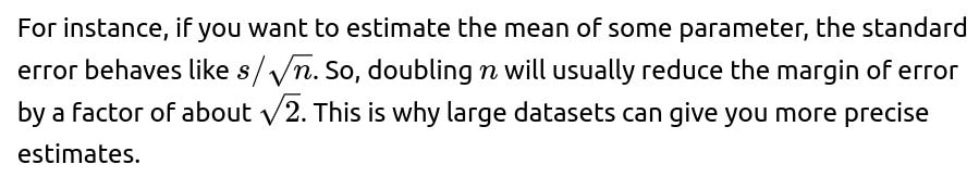
Diminishing returns: Even if you quadruple your sample size, the margin of error typically shrinks by half. Beyond a certain point, each additional data point might offer less benefit relative to cost.
How do you interpret confidence intervals in the presence of confounding variables?
Confounding variables can distort the relationship between the variable of interest and the outcome being measured. Even if you calculate a confidence interval around a sample mean or a coefficient in a regression, unaddressed confounders can produce misleading results because the parameter you’re estimating might not reflect the actual causal effect.
In observational studies, you often address confounders through methods such as stratification, multivariable regression, or propensity score matching. The confidence interval then applies to the adjusted parameter estimate. However, if there are unmeasured confounders, your interval might not capture the true effect, and no statistical method can fully compensate for missing or flawed data.
Potential pitfalls and edge cases
Unmeasured confounders: Even a seemingly tight confidence interval can be far from the real “truth” if a critical variable was omitted.
Residual confounding: Proper model specification is crucial; even if you measure confounders, an incorrect functional form (e.g., not modeling non-linear effects) can introduce bias.
Interpretation: A confidence interval in a regression output is conditioned on the correctness of the model. If key confounders are not included or are wrongly specified, the interval might give a false sense of precision.