
ML Interview Q Series: Confidence Intervals for Coin Toss Probability Using Normal Approximation

Browse all the Probability Interview Questions here.
How can you construct a confidence interval for the likelihood of getting heads when tossing a coin repeatedly?


Practical Implementation Example in Python
import math

def confidence_interval(num_heads, n, confidence_level=0.95):
    """
    Returns the (lower_bound, upper_bound) confidence interval
    for the probability p of flipping heads.
    Uses normal approximation to the binomial distribution.
    """
    # Calculate sample proportion
    p_hat = num_heads / n

    # Determine z-score for desired confidence level
    alpha = 1 - confidence_level
    # For 95% CI, z ~ 1.96. Here we can handle other levels by adjusting the lookup.
    # A quick approach (not recommended for mission-critical code):
    # dictionary could be used for common alphas or we can use scipy for a more accurate approach

    import scipy.stats as st
    z_value = st.norm.ppf(1 - alpha/2)

    # Standard error
    standard_error = math.sqrt(p_hat * (1 - p_hat) / n)

    # Margin of error
    margin_of_error = z_value * standard_error

    lower_bound = p_hat - margin_of_error
    upper_bound = p_hat + margin_of_error
    return (max(0, lower_bound), min(1, upper_bound))  # clip to [0,1] if desired

In such cases, the normal approximation can break down, and you might see intervals that include impossible probabilities (e.g., below 0 or above 1). A more robust approach is to use the Wilson score interval, which often yields better coverage properties even for smaller n. Another alternative is the “exact” Clopper-Pearson interval for the binomial parameter, which does not rely on large-sample approximations but can be more conservative.
Why do we rely on a z-score?
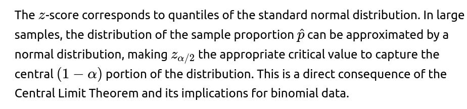
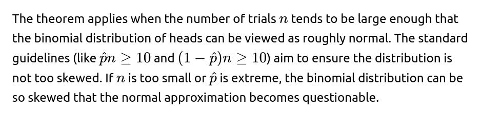
When does the Central Limit Theorem apply for proportions?

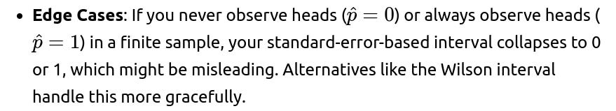
Potential Pitfalls and Real-World Considerations
Very High Confidence: If you demand a very high confidence level (e.g., 99.999%), your margin of error grows dramatically, sometimes rendering the result less informative.
Practical Relevance: Sometimes a confidence interval that is theoretically correct might still be too wide or too narrow to be useful in practice. Consider the cost of being wrong and the benefit of narrowing your estimates.
Sequential Testing: If you keep tossing the coin and re-checking the confidence interval as you go, you are effectively doing multiple tests, which can complicate your overall error rates.
Below are additional follow-up questions
What if the coin tosses are not truly independent?
If each toss is influenced by the outcome of previous tosses or by some external factor, the standard binomial assumption of independence between trials is violated. For example, suppose the probability of heads on a given toss might increase if the previous toss was heads, or perhaps the temperature in the room affects the coin’s balance. When dependence is introduced, the variance of the observed proportion may be larger or smaller than the nominal binomial variance.
A key pitfall is that even if you compute a standard confidence interval based on an assumption of independence, you might underestimate or overestimate the true variability. In practice, you could:
Use models that account for correlation, such as a Markov chain model if the dependence is sequential.
Estimate the effective sample size, which might be smaller than n if there is positive correlation among tosses.
Perform a block bootstrap or other resampling method that preserves correlation structure.
Real-world issues often arise in sensors or industrial processes where each measurement depends on the previous one. Failing to model correlation can lead to overly narrow (or occasionally overly wide) intervals that give a misleading sense of certainty (or uncertainty).
Can we construct Bayesian credible intervals for the probability of heads?
Yes, an alternative to frequentist confidence intervals is to use Bayesian credible intervals. The fundamental idea is to start with a prior distribution over p (the probability of heads), then update it with the observed data (number of heads in n tosses) to obtain a posterior distribution. A simple prior is the Beta distribution, often chosen because the binomial likelihood is a conjugate to the Beta prior, making the posterior also a Beta distribution.
A standard approach would be:

Choosing an inappropriate prior (e.g., one that heavily biases the result toward certain values).
Interpreting credible intervals incorrectly as frequentist confidence intervals (though in practice, they often have similar numerical values for large n).
Small-sample or heavily skewed data can produce wide or heavily biased posterior intervals if the prior parameters are chosen arbitrarily.
In real-world scenarios where domain expertise suggests strong beliefs about p (say, a coin is known to be fair or biased), a Bayesian approach can more directly incorporate this information and yield intervals that reflect prior knowledge plus observed evidence.
How can concept drift across the series of coin tosses affect the confidence interval?
Concept drift occurs if the true probability of heads changes over time—for example, a coin might get worn down or some external condition might alter its balance. If p is not constant during all tosses, then constructing a single confidence interval for a fixed p might be misleading.
Possible strategies include:
Segmenting the tosses into different time windows and computing separate estimates. You can see if p is shifting over time by comparing intervals in different segments.
Using a nonstationary statistical model, such as a time-varying parameter approach, to accommodate changes in p over the series.
If the drift is not too drastic, you might detect it by computing a rolling or cumulative estimate of p and see if it appears to systematically trend up or down.
A pitfall is failing to notice that the probability may be changing. This leads to intervals that neither reflect the earliest nor the latest state accurately. In real-world systems where parameters evolve (like evolving manufacturing processes), failing to detect and model drift can cause major miscalibration of intervals.
What if you need to construct intervals for multiple coins simultaneously?
When constructing intervals for multiple coins or multiple phenomena in the same experiment, you risk an inflated family-wise error rate if you interpret each interval independently at the same confidence level. This can lead to spurious findings about which coins are biased.
To address this:
Use adjustments like the Bonferroni correction or other multiple comparison controls (e.g., Holm’s method) to maintain an overall confidence level across all intervals.
Alternatively, consider hierarchical or Bayesian models that estimate multiple coins’ probabilities simultaneously, possibly sharing partial information.
A real-world issue arises if a researcher flips 100 different coins and tries to identify which ones are biased. Without adjusting for multiple comparisons, some coins will appear significantly “biased” just by chance alone. Ignoring multiple testing corrections can lead to false discoveries.
How does one handle rounding or discrete outcomes when reporting intervals?
In practical settings, you might report intervals only up to a certain decimal place or as percentages. Because p lies between 0 and 1, some intervals might get reported as, say, (0.00, 0.05), which can overstate how precise or imprecise the estimate really is. You might see intervals that round to [0.0, 1.0], which is not particularly informative.
Pitfalls include:
Over-rounding so that intervals become too coarse, losing nuanced information.
Reporting intervals that exceed [0,1] before rounding, which can confuse non-technical audiences if not clarified that the theoretical interval was clipped to [0,1].
In real-world scenarios, always check whether the final reported interval is still within plausible bounds and be transparent that any clipping or rounding can alter how the interval is perceived.
Is there a difference between confidence intervals for a proportion and prediction intervals?
Yes. A confidence interval for p describes uncertainty about the true underlying probability of heads. In contrast, a prediction interval describes uncertainty about future observations. For coin tosses, a prediction interval might address questions like: “Given our estimate of p, where do we expect the next batch of m coin tosses’ number of heads to lie?”
A subtlety is that a prediction interval must consider not only uncertainty in p but also the inherent binomial variability in the future outcomes. A pitfall is to confuse the two, assuming that a confidence interval for p is automatically describing how many heads you should expect in a future experiment. In real-world analyses, especially in risk assessment, it’s critical to distinguish between uncertainty in the parameter and the stochastic variability in new data.
Could an extreme outcome in a small sample skew the confidence interval significantly?
Yes. If you flip a coin only a handful of times and obtain unusual outcomes (e.g., 5 heads out of 5 flips), the normal approximation-based confidence interval might be very misleading, as it can erroneously place too much weight on the extreme result. You might end up with an interval near 1, but in reality, it was just a small sample. This scenario underlines:
The importance of using exact methods (e.g., Clopper-Pearson) or Bayesian priors that temper the effect of extreme results in small samples.
Real-world data often contain outliers or rare events, and you might erroneously generalize from a tiny set of observations.
A pitfall is concluding that the coin must be almost certainly double-headed. While a small-sample frequentist or Bayesian interval will indeed be influenced strongly by the data, having a prior (in the Bayesian context) can prevent you from concluding that p is close to 1 just because of a handful of flips.
Can the confidence interval approach be extended to account for measurement errors or misclassification in heads vs. tails?
If there is uncertainty about whether a flip was correctly recorded (for example, if sensors fail sometimes), then the simple binomial framework is incomplete. You now have a misclassification model or measurement error scenario. Strategies include:
Creating a latent variable model where the true state of each toss is never observed perfectly, but has some known or estimated probability of being misread.
Adjusting the likelihood function so it reflects not just Bernoulli(p) but Bernoulli(p) combined with conditional probabilities of misclassification.
A subtle pitfall is failing to account for repeated system misclassifications. If the sensor systematically overcounts heads, you can significantly bias your estimate of p. Real-world coin-flip-like experiments in labs or factories often face measurement errors, so it’s crucial to incorporate that in the model or else your confidence interval won’t represent the true probability of heads.