ML Interview Q Series: Constrained Optimization in ML: Using Projections and Lagrange Multipliers.

📚 Browse the full ML Interview series here.

Constrained Optimization: You need to optimize a model’s parameters under a constraint (for example, weights that must sum to 1 or be non-negative). How can you incorporate such constraints during optimization? *Describe an approach such as using Lagrange multipliers or projecting gradient updates to the feasible region.*

Approaches to Constrained Optimization involve modifying how gradient-based learning (or other optimization techniques) proceed, ensuring that candidate solutions always lie within or are actively pushed toward the feasible region. Constraints might be:

• Equality constraints (like parameters that sum to a constant).

• Inequality constraints (like parameters that must be >= 0).

Below are a few in-depth strategies to tackle such constraints.

Using Lagrange Multipliers

This approach augments the original objective function with additional terms that penalize (or enforce) the constraints.

We then optimize over both w and λ. We typically solve:

When dealing with inequality constraints, slack variables or KKT (Karush-Kuhn-Tucker) conditions can be introduced so that constraints such as h(w)≤0 are enforced. In deep learning frameworks, it can become numerically tricky or computationally heavy to solve these constraints directly within each mini-batch step. However, Lagrange multipliers remain theoretically elegant and form the basis for more sophisticated constrained optimization algorithms.

Projection Methods (Projected Gradient Descent)

Given a current parameter vector w, and a gradient-based update w←w−η ∇L(w), we then compute:

Key Insights and Real-World Examples

• Weights that must sum to 1 (Simplex constraint): Projection can be done by normalizing to ensure the sum equals 1 and all components remain non-negative.

• Non-negative constraints: Projection can be done by clipping negative values to zero after each update step.

• Positivity constraints in certain layers: For instance, in neural networks with physically meaningful parameters (like variances), or in attention distributions for certain specialized models, a projection step is used to ensure valid values.

• Lagrangian approaches with hyperparameter tuning: Lagrange multipliers might require scheduling or adaptively updating the multiplier to keep the constraint satisfied. This can be more complicated than a simple projection step but might give better theoretical or empirical results depending on the problem structure.

Example of Projected Gradient for Non-Negative Weights

Below is a minimal Python snippet illustrating how to incorporate a projection step to ensure weights stay non-negative. This is a toy example, not production-level code:

import torch

# Example: a simple parameter vector we want to keep >= 0
w = torch.tensor([0.5, -0.2, 1.2, 3.0], requires_grad=True)
learning_rate = 0.01

for iteration in range(100):
    # A dummy loss function: L(w) = sum(w^2)
    loss = (w ** 2).sum()

    # Compute gradients
    loss.backward()

    # Gradient step
    with torch.no_grad():
        w -= learning_rate * w.grad

    # Zero out the gradients for next iteration
    w.grad.zero_()

    # Projection step to ensure non-negativity
    w.clamp_(min=0.0)

# Now w is guaranteed to remain >= 0 after each iteration
print(w)

In a more general setting (like requiring w to lie on a simplex), the main difference is in how the projection is computed (e.g., you’d normalize by the sum of weights if you need them to sum to 1 and be non-negative).

Follow-up Question 1:

How exactly does one project onto the simplex if the weights must sum to 1 and remain non-negative?

When projecting onto a simplex, you typically:

1. Sort the weights in descending order.

2. Find the largest index k such that:

This ensures all projected components are non-negative and the total sums to exactly 1. In code, frameworks like PyTorch don’t have a built-in “simplex projection” operation by default, so you generally implement this procedure manually or rely on common libraries that do it for you. The key concept is to shift each coordinate by the same amount so that the sum becomes 1, while simultaneously clipping at zero for negativity constraints.

Follow-up Question 2:

Are there any caveats when using Lagrange multipliers in large-scale machine learning problems?

Yes, there are multiple caveats:

• Stability and Convergence Issues: Solving for the multipliers in each mini-batch might be unstable if done naively. You may need adaptive or approximate methods (e.g., primal-dual methods or penalty methods).

• Computational Overhead: Updating or solving for the Lagrange multipliers in every iteration can be expensive, especially if constraints are complex. For high-dimensional parameter spaces, solving these systems can be non-trivial.

• Hyperparameter Tuning of the Multiplier: You might have to tune the Lagrange multiplier’s learning rate or schedule. If the multiplier is too large, it may dominate and stall progress. If it’s too small, the constraint may not be enforced well.

Follow-up Question 3:

What if I have inequality constraints that require a parameter to stay within a range, such as [a, b]? How do I incorporate that during training?

One of the easiest approaches is to do a projection step that clips parameters within the specified range. For every gradient update, you do:

1. Gradient-based update of the parameter.

2. Projection by clamping to the range [a, b].

This ensures parameters never leave that interval. If you want to handle it via Lagrange multipliers, it becomes a KKT conditions scenario, and you typically handle it via specialized solvers or incorporate penalty terms. But in many practical deep learning tasks, a simple clamp or a reparameterization can be sufficient. Reparameterization is another approach where you might set w=a+(b−a) σ(θ), ensuring w always lies between a and b. Then you optimize θ unconstrained, using standard gradient methods. This is a neat trick in many real-world neural network layers that require bounded parameters.

Follow-up Question 4:

When is it preferable to use a reparameterization trick rather than a projection approach?

Reparameterization is often used when:

• You want smooth, differentiable updates that never require abrupt operations like clipping.

• You want to avoid repeated computations of a projection operator (which could be computationally expensive for complex constraints).

• You’d like to incorporate constraints in a way that the parameter space is unconstrained (making optimization simpler in certain contexts).

• You want your parameterization to have direct interpretability. For example, if you ensure a parameter is always positive by using an exponential transform w=exp⁡(θ), you can then interpret changes in θ as multiplicative changes in w. Clipping might lose that direct interpretability.

However, if your feasible region is complicated or if you do not want to transform your entire parameter space, projection can be simpler. The best choice depends on the computational cost and the geometry of the constraint set.

Follow-up Question 5:

What are some pitfalls of projecting weights, say onto the simplex, for neural network models?

• Loss of Gradient Information: Projection steps can be abrupt. If a parameter moves far outside the simplex, a large chunk of gradient information is “thrown away” during projection.

• Non-smoothness: Projection is sometimes non-differentiable at boundary points. In practice, this can slow or complicate convergence.

• Slower Convergence in Some Cases: If the true optimum lies near a boundary, repeated projection might cause large oscillations.

• Implementation Complexity: Simplex projection is a more involved procedure than the typical “clip” function. Mistakes in implementation can lead to subtle bugs.

Despite these pitfalls, projection-based methods remain widely used due to their simplicity and directness in ensuring feasible solutions after each update.

Follow-up Question 6:

Can you provide a more detailed code snippet illustrating a simple PyTorch training loop with a projection step to ensure weights stay on the simplex?

Below is an illustrative example for a single layer (weights are 1D for simplicity). In a real neural network scenario, you’d adapt this logic to the relevant parameters or layers.

import torch
import torch.nn as nn
import torch.optim as optim

def project_simplex(v):
    """
    Projects a PyTorch 1D tensor v onto the probability simplex.
    Ensures sum of elements = 1, all elements >= 0.
    """
    # Sort v in descending order
    sorted_v, indices = torch.sort(v, descending=True)
    # Compute the cumulative sum
    cumsum = torch.cumsum(sorted_v, dim=0)

    # Determine the rho
    # We find the largest k such that sorted_v[k] - (1/k)*(sum_{j=1 to k}(sorted_v[j]) - 1) > 0
    rho = torch.where(sorted_v - (1.0 / torch.arange(1, len(v) + 1, device=v.device)) * (cumsum - 1) > 0)[0]
    if len(rho) == 0:
        rho_val = 0
    else:
        rho_val = rho[-1].item()

    # The threshold
    theta = (cumsum[int(rho_val)] - 1) / (rho_val + 1)

    # Perform the projection
    w = torch.clamp(v - theta, min=0)
    return w

# A simple linear model with 4 parameters
class SimpleModel(nn.Module):
    def __init__(self):
        super(SimpleModel, self).__init__()
        self.params = nn.Parameter(torch.rand(4))  # random init

    def forward(self, x):
        # Just a dummy forward to illustrate usage
        # Weighted sum of input
        return (x * self.params).sum(dim=1)

# Dummy dataset
X = torch.randn(100, 4)
y = torch.randn(100)

model = SimpleModel()
optimizer = optim.SGD([model.params], lr=0.1)

for epoch in range(10):
    optimizer.zero_grad()
    preds = model(X)
    loss = ((preds - y) ** 2).mean()
    loss.backward()

    # Normal gradient step
    optimizer.step()

    # Projection step onto the simplex
    with torch.no_grad():
        model.params.data = project_simplex(model.params.data)

    # Check the sum of params
    print(f"Epoch {epoch}: loss={loss.item()}, sum_of_params={model.params.data.sum().item()}")

In this snippet:

• We have a single parameter vector model.params.

• After each gradient update, we call project_simplex to ensure that the new parameter vector sums to 1 and remains non-negative.

• This ensures feasible updates throughout training.

Follow-up Question 7:

Are there scenarios where a penalty-based approach might be preferable to projection or direct Lagrange multipliers?

• Is straightforward to implement in modern deep learning frameworks (just define the penalty inside the loss).

• Allows a soft constraint, letting the model occasionally violate it if that leads to better optimization progress, but eventually, the penalty cost becomes large.

• Might be less exact than a strict projection or direct Lagrange approach, because the final solution can still violate the constraint slightly if the penalty is not huge enough.

In practice, you can treat the penalty coefficient as a hyperparameter. If you set it very large, you push the solution close to the constraint. If it’s too large, training might become unstable. If it’s too small, your constraint might be loosely enforced.

Follow-up Question 8:

What about using external optimizers that can handle constraints directly, like certain variants of constrained optimization solvers?

For some specialized tasks—especially smaller-scale problems—you could use methods such as Sequential Quadratic Programming (SQP), interior-point methods, or augmented Lagrangian methods that come packaged in libraries like SciPy (scipy.optimize.minimize with constraints). However, these methods might be too slow for large-scale deep learning because they often require multiple passes over the dataset to compute Hessians or Hessian approximations and do sophisticated line searches.

In big neural network training:

• Stochastic gradient-based methods with straightforward projection or reparameterization are typically favored.

• Full-blown constrained optimization routines might be used in smaller or specialized tasks where constraints are extremely important (e.g., scientific computing, calibration tasks, or certain portfolio optimization in finance).

The choice largely depends on the size of the problem, the type of constraint, and how critical it is to strictly satisfy it at each iteration.

Follow-up Question 9:

Could you elaborate on KKT conditions and how they generalize Lagrange multipliers for inequality constraints?

Karush-Kuhn-Tucker (KKT) conditions extend the idea of Lagrange multipliers to handle inequality constraints:

These conditions ensure a consistent solution that satisfies the constraints. In deep learning or general large-scale settings, we rarely solve KKT conditions explicitly in each iteration because it can be computationally intense. Instead, we approximate them via methods like projected gradient descent or by adding penalty terms and letting standard optimizers find approximate solutions that eventually respect the constraints.

Follow-up Question 10:

In practice, do methods like projecting gradients or using reparameterization have any significant performance cost or difficulty integrating with modern frameworks like PyTorch or TensorFlow?

• Performance Cost: Usually small, especially if the projection is a simple clamp or straightforward normalization. More advanced projections (like onto complex polyhedral sets) might add overhead, but typically it’s not large relative to overall training time.

• Integration Difficulty: Minimal with clamp-based or reparameterization approaches. Frameworks like PyTorch or TensorFlow are flexible, allowing custom operations right after gradient updates. The only subtlety is ensuring these steps don’t mess up gradient tracking. Usually, you wrap them in a torch.no_grad() or use an optimizer hook to handle the projection.

• Reparameterization Overheads: Just a matter of how you define your parameters. If you do something like w=exp⁡(θ), that’s just a standard exponential operation on a trainable parameter θ. This is well-supported and has negligible overhead. However, if your constraint set is complicated, the reparameterization might be more involved.

Hence, for constraints like “weights sum to 1” or “weights >= 0,” these methods tend to be both conceptually simple and computationally cheap.

Follow-up Question 11:

Are there any specific domain applications where constrained optimization is particularly prevalent?

• Portfolio Optimization in Finance: Weights typically must be non-negative and sum to 1.

• Probability Modeling: If a parameter vector represents a probability distribution (like attention weights or mixture components), it must lie on a simplex.

• Resource Allocation Problems: Allocating limited resources subject to capacity constraints often requires ensuring feasible solutions.

• Physical Models: In engineering or physics-based models, certain parameters must be positive to be physically meaningful (e.g., time constants, masses, conductances).

• Hyperparameter Constraints: In Bayesian hyperparameter tuning, you might constrain hyperparameters to ensure valid priors or distributions.

In all such settings, using projection methods, reparameterization, or penalty-based approaches is a practical solution integrated into existing frameworks.

Follow-up Question 12:

How do you decide between direct Lagrange multiplier approaches, projection methods, penalty-based methods, or reparameterization in practice?

It often boils down to these considerations:

• Complexity of Constraint: If constraints are straightforward (like positivity or simplex), projection or reparameterization is typically the first choice. If constraints are more complex (like multiple simultaneous equality and inequality constraints), penalty or Lagrangian approaches might be required.

• Ease of Implementation: Projection and reparameterization can be easier to code, especially in iterative deep learning loops.

• Exactness vs. Softness of Constraint: If the constraint is strict, and any violation is unacceptable, projection or a large penalty might be used. If small deviations are tolerable, a moderate penalty can suffice.

• Computational Cost: Lagrange multiplier updates or advanced constrained optimizers can be more expensive, so in large-scale problems, simpler methods typically dominate.

• Stability: Reparameterization methods often provide more stable gradients since everything remains differentiable, whereas projection can cause abrupt changes at the boundary. Lagrange multipliers can be tricky to tune.

Ultimately, the decision is often an empirical one in the deep learning community, with preference given to whichever method is simpler to deploy and stable in training while still meeting the constraint requirements.

Follow-up Question 13:

Is there any recommended best practice for logging or monitoring constraints during training?

Yes. You generally want to track:

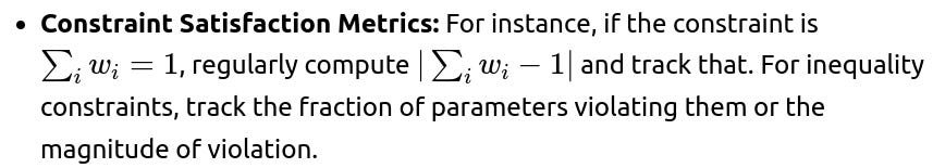
• Effect of Constraint on Loss: Observing whether the model’s main loss is being negatively impacted by the constraint can be informative.

• Lagrange Multiplier Magnitude (if using Lagrangians): See if multipliers blow up or vanish, which indicates instability or irrelevance of certain constraints.

In standard deep learning frameworks, you log these metrics in TensorBoard or a similar monitoring tool to ensure the constraint is respected and the overall optimization is proceeding as intended.

Follow-up Question 14:

How do these methods generalize to multiple constraints?

• Lagrange Multipliers: Introduce one multiplier per constraint, leading to a system of equations or a more complex primal-dual approach.

• Projection: If the constraint set is the intersection of multiple sets, you might need an iterative method like Dykstra’s projection or more advanced algorithms, because projecting onto each constraint set individually and sequentially might be necessary.

• Penalties: Sum up penalty terms for each violation.

• Reparameterization: Potentially more complicated if the feasible set is defined by multiple intricate constraints, but still possible with advanced transforms.

Each approach’s complexity grows with the number of constraints, so in deep learning, people often keep constraints as simple as possible.

Follow-up Question 15:

Is there a method to handle constraints that change over time during training, such as time-varying constraints or constraints that become tighter as training progresses?

You can adapt many methods dynamically:

• Projection: If your constraint set changes each epoch, you just project onto the updated set.

• Lagrange Multipliers: The multipliers can be updated iteratively, so if constraints become tighter, the multipliers might become bigger to enforce them.

• Penalty-based: Dynamically scale up the penalty coefficient so that constraints become stricter over time. For instance, start with a moderate penalty and increase it across epochs to let the network explore solutions but gradually enforce the constraint more strongly.

This kind of schedule is sometimes used in curriculum learning or in domain adaptation scenarios where constraints represent environment changes.

Follow-up Question 16:

What common mistakes do people make when implementing projection-based gradient methods?

• Failure to Disable Gradient Tracking During Projection: You often want to apply the projection as a post-processing step that doesn’t backprop through the projection itself, unless you explicitly intend to incorporate that derivative. If you don’t use with torch.no_grad():, you can end up with odd behaviors or computational graph issues.

• Incorrect Implementation of Projection Operator: Especially for simplex or more complex sets, it’s easy to accidentally implement the algorithm incorrectly, leading to a projected vector that doesn’t truly lie in the feasible region.

• Ignoring the Potential for Zero Gradients at Boundaries: If your parameters frequently hit boundaries, the gradient steps might produce suboptimal updates. This can cause training stalling or weird plateaus.

• Infrequent Projections: Some might only project occasionally (say every 10 steps) rather than every step, which can let the parameters drift outside the feasible region for too long and cause instability.

Follow-up Question 17:

Would using a built-in layer or parameter initialization that inherently satisfies constraints remove the need for projection entirely?

Potentially, yes. For instance:

• Using a softmax layer ensures non-negative outputs that sum to 1 automatically. This is effectively a reparameterization that transforms unconstrained parameters into a simplex.

• Using an exponential transform ensures positivity.

• Using a sigmoid transform ensures the parameter stays in [0, 1].

This approach is quite common in neural networks: feed the raw parameter θ through a function f(θ) that enforces the constraint, and treat θ as the actual trainable parameter. Then you don’t need an explicit projection step. The choice depends on your objective function and how naturally you can incorporate these transformations.

Below are additional follow-up questions

How does constrained optimization interact with normalization layers such as BatchNorm?

Normalization layers adjust intermediate activations, not the raw model parameters themselves (e.g., weight matrices), so they rarely conflict directly with constraints placed on model parameters. However, there are subtle points to consider:

• Impact on Effective Parameter Distribution: If your constrained parameters feed into a BatchNorm layer, the layer will normalize the outputs. Even if your parameters are constrained to be non-negative, BatchNorm might shift or scale those activations into negative ranges or beyond. If your constraint was meant to enforce certain sign or scale properties of intermediate outputs (rather than weights), you must ensure the normalization does not violate your high-level objective for bounding those outputs.

• Training Stability: Normalization layers attempt to maintain stable distributions of activations. If you impose strict constraints (like projecting onto a simplex or clipping to [0, 1]), there is a possibility that the combined effect with BatchNorm’s re-centering can lead to unexpected behavior or slower convergence. You might see extra fluctuations in early epochs if your feasible set is small or if constraints and normalization are fighting each other.

• Practical Workaround: Often, constraints on model parameters are relatively orthogonal to BatchNorm. For instance, if your parameters must stay on a simplex, you just project them after each optimization step. BatchNorm will still do its job, adjusting means and variances of forward-pass activations. In practice, training is usually stable, though you should monitor metrics to ensure constraints remain satisfied and that normalization is not amplifying boundary effects.

• Edge Cases: If you attempt to constrain the scale or sign of BatchNorm’s own learnable parameters (the “gamma” and “beta”), you must incorporate separate projection or reparameterization for them as well. This can be relevant if your model architecture specifically requires controlling these normalization parameters for interpretability or physical consistency.

Thus, in typical usage, constraints on weights coexist without major issues. Just be vigilant if your constraints aim at controlling certain activation properties that might be confounded by normalization layers.

If the constraint is on intermediate computations rather than final weights, how do we handle that?

A constraint might apply to outputs of particular layers (e.g., a hidden state must remain above zero for interpretability or safety). This differs from constraining the learned weight parameters directly. Possible strategies include:

• Reparameterizing the Intermediate Output: Instead of letting the layer output arbitrary values, pass the pre-activation through a transform that enforces your constraint. For example, if you need non-negative intermediate activations, you could replace the linear or convolution layer’s activation with a softplus or ReLU. This naturally enforces positivity.

• Projection in the Computation Graph: If you can’t change the activation function, you might do a projection step inline for each forward pass. This is more unusual and can become computationally expensive or complicated, because you’re projecting large tensors rather than just a small set of parameters.

• Penalty Methods for Intermediate Outputs: You could add a term in your loss function that penalizes negative values (if your constraint is non-negativity) or penalizes any violation of your specified condition on the intermediate layer output. The model will learn to keep that penalty small, effectively respecting the constraint in practice. This approach is simpler to implement but only enforces a “soft” constraint.

A subtlety is that projecting or reparameterizing large activation tensors can disrupt gradient flow or degrade performance if done incorrectly. Testing and validation on realistic data distributions are important, as constraints on intermediate states can cause unexpected saturation, vanishing gradients, or mismatches with normalization steps.

How can fairness or societal constraints be incorporated into the optimization?

Fairness constraints often require certain statistical measures (e.g., equalized odds, demographic parity) to hold across subgroups. Incorporating these constraints can be more complex than simpler constraints like non-negativity. Options include:

• Lagrangian Approach on Fairness Metrics: Define a fairness violation function (e.g., difference in false-positive rates between groups) as a constraint. Introduce a Lagrange multiplier that penalizes any deviation from the fairness target. You periodically estimate fairness metrics on mini-batches or entire validation sets, then update multipliers to enforce the constraint. This can be computationally heavy because fairness metrics typically require label predictions aggregated by group membership.

• Post-Processing or Projection of Predictions: Instead of restricting model parameters, some fairness algorithms project final predictions (probabilities) onto a feasible fairness region. For instance, you might adjust predicted probabilities so that a specified average acceptance rate is enforced across subgroups. This is akin to a projection step but applied to predictions rather than model weights.

• Adversarial Training: Another approach is to train an auxiliary adversary that tries to detect protected attributes from model predictions or representations. Minimizing adversary performance can enforce a form of fairness. This is not a strict constraint in the sense of a direct equality or inequality, but it aims to remove sensitive information in a systematic way.

• Pitfalls: Fairness metrics are often discrete and can require multiple passes over data to compute. This can clash with stochastic optimization. Also, real-world definitions of fairness can be conflicting (equalized odds vs. demographic parity), so specifying the correct constraint is itself a domain challenge. Implementation details (like accurate subgroup sampling or weighting in mini-batches) are critical to success.

In practice, many fairness constraints are enforced in a hybrid manner: partial constraints or penalties integrated with standard training, plus post-processing adjustments.

Are there performance or memory overhead considerations when scaling constraints to large networks?

Large-scale neural networks, especially those with tens or hundreds of millions of parameters, can be sensitive to any additional overhead in the training loop. Key considerations:

• Projection Complexity: Certain projection operators (e.g., projecting onto a simplex or more complex polyhedra) may require sorting large parameter vectors. Sorting can be expensive at scale, so it might slow training if done naively in each step.

• Parameter Slicing: A possible optimization is to group parameters into smaller segments if the constraints apply independently to different subsets (e.g., each row of a weight matrix). This can reduce sorting overhead. Alternatively, you might do partial or approximate projections if an exact solution is too costly.

• Memory Overhead: If you must store additional buffers or multipliers for each parameter, memory consumption could rise significantly for large models. Lagrange multiplier approaches might require persistent multiplier states. Penalty methods can be more memory-friendly if you simply add terms to the loss without storing many additional tensors.

• Efficient Parallelization: In distributed training, you might need to coordinate across multiple GPUs or machines to ensure consistent projection steps. Communication overhead can increase if constraints are computed globally.

Ultimately, the practicality of constraints depends on how demanding the operations are relative to your overall training budget. Many simple constraints (clamping to [0, 1]) have negligible overhead, but advanced constraints (simplex projection across large parameter sets) might be non-trivial to scale.

What if the model parameters are stored on GPUs? Do we need special handling for projection or Lagrange multiplier updates?

Modern deep learning frameworks handle GPU memory seamlessly as long as your constraint operations are written in a way that can run on GPU. Here are subtle points:

• Implementation on GPU: Most array operations (like sorting, clamping, etc.) have GPU-compatible implementations in libraries like PyTorch and TensorFlow. If you rely on a custom CPU-based function for projection, transferring data back and forth between CPU and GPU each iteration can become a bottleneck. Implementing it fully on GPU is usually preferred.

• Atomic Operations in Distributed Settings: If you do synchronous gradient updates across multiple GPUs, ensure that your constraint step is consistently applied after the global aggregation of gradients. Otherwise, you might end up with race conditions where each GPU’s local projection conflicts with the final aggregated parameter state.

• Precision Issues: On some GPUs, floating-point precision is limited (especially if using mixed precision training). Projecting onto certain sets that require high numerical accuracy (like enforcing an exact sum of 1) might introduce rounding or small drifting. Usually, this is negligible, but for highly sensitive tasks, double-check the numerical stability.

Overall, as long as your projection or multiplier updates are GPU-friendly, you typically do not need fundamentally different logic. Just be mindful of data transfer and concurrency.

Can constraints reduce the expressive power or capacity of a deep model?

Yes, constraints can restrict the model’s parameter space, which may reduce expressivity:

• Excessive Restriction: For instance, forcing a large portion of parameters to remain non-negative could hamper the network’s ability to represent certain functions. Some tasks benefit from having both positive and negative weights, especially in gating or skip-connection contexts.

• Trade-off with Interpretability: Constraints often improve interpretability (e.g., probability distributions, physically meaningful parameters), but that might come at the cost of raw predictive power. If your domain strongly demands constraints (like safety-critical systems), the trade-off is usually acceptable.

• Workarounds: If you suspect a constraint is too strict, you can consider “soft constraints” via penalties, or reparameterization that slightly broadens the feasible region. Sometimes, partial constraints (constraining only certain layers) are enough to achieve the desired property while preserving overall capacity.

Despite potential capacity reductions, constraints can also act as useful regularizers. By eliminating extreme or physically implausible parameter configurations, constraints may improve generalization in practice.

How do we handle discrete or integer constraints on parameters?

Integer constraints present a unique challenge because standard gradient-based methods assume continuous parameters:

• Continuous Relaxation: Often you relax integer constraints to a continuous approximation, train with gradient-based methods, then round to integers post hoc. This is common in neural network quantization or embedding lookups. The final rounding step might degrade performance, but it’s often the simplest approach.

• Gumbel-Softmax or Straight-Through Estimator: If you need discrete parameters that represent categories (e.g., a parameter that must be one-hot), you can use a continuous approximation such as Gumbel-Softmax during training to allow backpropagation, then discretize at inference. This is effectively reparameterization for discrete variables.

• Integer Programming Approaches: For small-scale problems, one might use specialized integer programming solvers, but this is typically not feasible for large-scale deep networks. The overhead is enormous, and you lose the efficiency of standard GPU-based backprop.

• Mixed Strategies: Some tasks do repeated forward passes with different discrete parameter settings if the search space is small, or use reinforcement learning methods to treat discrete parameter choices as actions with a reward. This can be an indirect approach to constrained optimization.

Overall, integer or discrete constraints are far more complex than standard inequality/equality constraints. Practical usage in large neural networks often relies on relaxation or specialized approximation techniques.

Could constraints introduce instability in distributed or asynchronous training scenarios?

In distributed training, multiple workers or GPUs compute gradients independently and then synchronize updates. Constraints can introduce added complexity:

• Asynchronous Updates: If each worker projects parameters locally before synchronization, conflicting projections may lead to oscillations. One worker’s projection might push parameters to a boundary while another worker’s gradient step pulls them away.

• Consistent Constraint Enforcement: A robust approach is to aggregate gradients first (e.g., via an all-reduce), perform one consolidated update, and then apply the projection step or Lagrange multiplier update exactly once. This ensures consistency.

• Scaling of Lagrange Multipliers: In large-scale data parallelism, each worker might compute partial constraints or partial penalty terms. You must coordinate the multipliers or aggregated penalty signals across all workers. Failing to do so could lead to partial or incorrect constraint enforcement.

• Pitfalls in Monitoring: If constraints are enforced partially on each worker’s subset of data, you might never see a global violation until after many updates. Similarly, local mini-batches might not represent the entire distribution, so local constraint satisfaction doesn’t guarantee global satisfaction.

Hence, in distributed settings, it’s crucial to treat constraint steps as global operations, or carefully design them so local constraint checks align with the overall objective.

How do popular optimizers like Adam or RMSProp interact with projection or reparameterization?

Popular adaptive optimizers compute parameter-wise learning rates using past gradients. This can interact with constraints in a few ways:

• Projection after Adam Step: You can still do your usual Adam update, and then project to enforce constraints. Adam’s adaptive step might cause larger or smaller updates for certain parameters, but the subsequent projection can override these. If the step is significantly outside the constraint region, the projection might discard a substantial portion of the adaptive gradient. This could lead to suboptimal usage of Adam’s momentum or second-moment estimates.

• Reparameterization with Adam: If you reparameterize such that your constrained parameter w is an exponential or sigmoid transform of an unconstrained parameter θ, Adam will optimize θ. This typically works well, and you get the benefits of adaptive learning rates without explicitly projecting w. The only difference is you must track θ in your optimizer’s state.

• Hyperparameter Tuning: The combination of adaptive optimizers and constraints can require a different learning rate schedule or different beta parameters. Constraints might reduce the feasible step size or cause frequent boundary hits, so you might need a smaller learning rate or more frequent projection.

• Pitfall in Sums-to-1 Constraints: If you’re using a projection onto the simplex, Adam’s per-parameter adaptation might not necessarily “respect” the fact that all parameters are linked by the equality constraint. That is, a large adaptive step on one parameter could push it far out of the simplex, forcing an aggressive projection that discards nuance from the Adam updates. A well-tuned learning rate often mitigates this.

Still, Adam plus a projection or reparameterization is common in practical scenarios and usually yields stable results with some tuning.

If the data distribution changes over time (e.g., non-stationary or streaming data), can constraints adapt on the fly?

Yes, though you must decide how dynamic constraints should be enforced:

• Time-Varying Constraint Sets: If constraints tighten or shift as new data arrives, your projection operator or penalty function must be updated accordingly. For example, if you have a maximum-likelihood model with a physical constraint that changes with external conditions, you update the feasible set before each training epoch.

• Lagrange Multiplier Updates: If you’re using a Lagrangian approach, multipliers can be adapted or re-initialized when constraints change. You might need to re-warm your multipliers if the feasible region drastically shifts, or else you risk large, abrupt updates that destabilize training.

• Online Learning Considerations: In streaming scenarios, you typically do small incremental updates. Quick projection steps or reparameterization remain feasible. However, if your constraint set changes unpredictably, you must ensure your model can smoothly transition without repeatedly stepping far outside the feasible region.

• Pitfalls: If constraints fluctuate rapidly, your model parameters might bounce around boundaries or frequently get projected back, preventing stable convergence. Sometimes, a softer penalty-based approach can yield smoother transitions by not enforcing the constraints too rigidly in each mini-batch.

Hence, constraints can adapt, but you should carefully design the mechanism for updating them, particularly in real-time or streaming environments.

How might constraints be integrated with advanced techniques like Bayesian neural networks or variational inference?

In Bayesian or variational settings, you maintain a distribution over parameters rather than a single point estimate:

• Constrained Variational Distribution: If your parameter space is constrained (e.g., each parameter in a simplex), you might choose a variational family that inherently respects those constraints. For instance, a Dirichlet distribution for parameters that must lie on a simplex. Then you learn the Dirichlet’s concentration parameters. This is effectively reparameterization at the distribution level.

• Projection in Parameter Samples: If you sample parameters from an unconstrained distribution but want each sample to satisfy constraints, you could project the samples. However, this can introduce a mismatch between the distribution you’re sampling from and the final feasible region.

• Penalties on the Distribution: In a hierarchical or Bayesian approach, you might incorporate constraints as priors that heavily favor feasible regions. For example, a prior that enforces positivity can be an exponential or half-normal prior. This keeps the posterior in the feasible region without explicit projection each time.

• Computational Complexity: Bayesian methods are already more computationally intensive. Adding constraints (especially complicated ones) can further increase the cost or reduce the availability of closed-form solutions for posterior updates. Approximate sampling or specialized inference algorithms might be needed.

In practice, the exact method depends on how strictly you need to enforce constraints within the Bayesian framework. Many times, a well-chosen prior suffices to keep parameter draws in a plausible region without explicit projection steps.

Can constraints help in regularizing or preventing overfitting in certain tasks?

Yes, constraints can act similarly to regularizers:

• Physically Meaningful Constraints as Inductive Bias: For example, in modeling growth processes, you might constrain model outputs to be non-decreasing over time. This integrates domain knowledge and can reduce spurious solutions.

• Trade-off with Model Flexibility: Over-constraining can underfit if the model cannot capture the data complexities. A sweet spot often emerges, where constraints provide beneficial inductive bias without overly restricting the solution space.

• Practical Implementation: In deep learning tasks like attention mechanisms, ensuring attention distributions sum to 1 naturally interprets them as probabilities, which can lead to more robust interpretability and sometimes better generalization. Similarly, non-negativity constraints for certain gating parameters can reduce degenerate solutions.

Hence, constraints can be viewed as a form of domain-inspired regularization, helping steer the network towards plausible or interpretable solutions.

How do we debug a situation where adding constraints causes the model to diverge or fail to train?

Debugging approaches:

• Check Gradients: Observe if gradients explode or vanish after the projection step. Large norm differences before and after projection might indicate the learning rate is too high or the projection is too severe.

• Inspect Constraint Satisfaction Over Time: Log how closely the model meets constraints each epoch. If it frequently violates them by large margins, or if the Lagrange multiplier or penalty term becomes huge, the training loop might be stuck in a tug-of-war between the objective and the constraints.

• Use Simplified Constraints or Lower-Dimensional Tests: Test your method on a small toy problem where the parameter dimension is low (e.g., 2D or 3D). Visualize the constraint set and the trajectory of the optimization to see if it’s stepping outside in a strange pattern.

• Reduce Learning Rate or Projection Frequency: Sometimes applying projection every step can be too abrupt. You might reduce the frequency (though it risks partial violations) or reduce the learning rate so updates remain in the feasible region more gently.

• Check for Implementation Bugs: Mistakes in projecting onto complex sets (like incorrectly sorting in simplex projection) or forgetting to disable gradient tracking during the projection can produce bizarre training behaviors.

• Try a Different Constraint Method: If a Lagrange multiplier approach is unstable, a simpler penalty-based or reparameterization approach might converge more smoothly. Conversely, if penalty methods fail to enforce constraints strictly enough, a direct projection might be necessary.

Thorough logging and step-by-step analysis are key. As constraints add another layer of complexity, debugging often requires carefully isolating each part of the pipeline (objective, constraints, and optimizer) to identify where the instability arises.

Could constraints break gradient flow if not implemented carefully?

Absolutely. Certain operations can inadvertently block or alter gradients in unintended ways:

• Clamping or ReLU-Style Projections: Hard clipping to a boundary at zero can zero out gradients for parameters that land exactly on the boundary. If a parameter is consistently pinned at zero, it might never move away. This is sometimes desired (staying on the boundary) but can hamper learning if the boundary is frequently reached.

• Stop-Gradient Errors: In frameworks like TensorFlow or PyTorch, if you apply the projection step within the computational graph without properly handling gradient flow, the backprop might not propagate through the projection (depending on the function). Often, you want the projection to be outside the gradient flow, but you must confirm your intention.

• Using Non-Differentiable Constraints: Projection operators can be non-differentiable at corners or edges of the feasible set. This might cause subgradient or no gradient at those points, potentially making training less smooth or more prone to local minima.

In practice, reparameterization strategies are often preferred if you want fully differentiable flows. If you need a strict projection, you must accept that boundary conditions can cause abrupt changes in gradient behavior.

Does the feasibility of solutions become an issue when multiple constraints are contradictory or very tight?

Yes, feasibility can become a significant problem:

• No Feasible Solution: If constraints are impossible to satisfy simultaneously, training might fail altogether. For example, if you have two equality constraints that sum to contradictory values, no parameter can satisfy both.

• Overconstrained Scenario: If the constraints are extremely tight, the model might effectively have few degrees of freedom left. You could end up with near-zero training loss improvement because almost every gradient step is undone by the projection to a tiny feasible region.

• Detecting Infeasibility: When using Lagrange multipliers, multipliers might blow up, or the optimization might diverge, suggesting the constraints cannot be simultaneously satisfied. With projection-based methods, you might see the projection snapping you to an extreme corner with zero improvement. Logging metrics that reflect constraint violation is essential for diagnosing this early.

• Relaxation or Prioritization: Real-world problems sometimes rank constraints by importance. If certain constraints are more flexible, turn them into soft penalties while strictly enforcing the crucial ones. Alternatively, you can systematically relax constraints by a small margin to ensure a feasible region exists.

Balancing contradictory or extremely tight constraints usually requires domain-specific compromises or advanced multi-objective optimization methods.

Are there library/tooling solutions that automate constrained optimization in deep learning?

While not as common as unconstrained frameworks, there are some libraries and approaches:

• PyTorch Ecosystem: Several user-contributed libraries implement simplex projection or specialized reparameterization modules. PyTorch itself does not have a built-in constrained optimizer API, so you typically code the constraints manually or rely on a specialized extension.

• TensorFlow Addons or Custom Keras Callbacks: Similar approach. A callback might implement a post-update projection step or a custom training loop that integrates constraints.

• OptNet / Differentiable Optimization Layers: Some research libraries embed differentiable optimization solvers into neural networks, allowing constraints to be enforced by an internal solver that is part of the forward pass. This can handle certain linear or quadratic constraints. However, it’s more niche and can be costly for large-scale tasks.

• SciPy or JAX Libraries: SciPy’s optimize.minimize can handle constraints but is primarily CPU-based and not designed for deep networks at scale. JAX has some advanced transformations that might facilitate partial integration of constrained optimizations, but again, large-scale usage can be complex.

Most practitioners implement their own constraints or reparameterizations due to the simplicity and flexibility required in typical deep learning workflows. The community is gradually evolving more advanced tooling, but it remains a specialized need relative to the majority of unconstrained use cases.