
ML Interview Q Series: Constructing Correlated Bivariate Normals via Linear Transformation of Independent Normals.
Browse all the Probability Interview Questions here.
Constructing Correlated Bivariate Normals via Linear Transformation of Independent Normals.


Short Compact solution
For any real constants a and b, the linear combination aX + b(ρX + √(1−ρ²)Z) is itself a linear combination of X and Z. Because X and Z are independent and normally distributed, any such linear combination is also normally distributed. By computing the means, variances, and covariance, we verify that the new pair (X, ρX + √(1−ρ²)Z) has zero mean, unit marginal variances, and correlation ρ. Hence it is a standard bivariate normal with the same parameters as (X, Y).
Comprehensive Explanation
Verifying Normality
One key fact about normally distributed variables is that any linear combination of jointly normal random variables is also normally distributed. In our setting, X and Z are independent and both follow N(0,1). The pair (X,Z) is therefore bivariate normal. If we define V = X W = ρX + √(1−ρ²)Z, then (V, W) is still a bivariate normal vector because V and W are each linear combinations of the jointly normal pair (X, Z).
Mean and Variance Calculations
We next check the means and variances to confirm they match the standard bivariate normal specification with correlation ρ.
E(V) = E(X). Since X ~ N(0,1), E(X) = 0. Thus E(V) = 0.
E(W) = E(ρX + √(1−ρ²)Z) = ρ E(X) + √(1−ρ²) E(Z). Both X and Z have mean 0, so E(W) = 0.
Var(V) = Var(X) = 1.
Var(W) = Var(ρX + √(1−ρ²)Z). By independence of X and Z and their unit variances, we get Var(W) = ρ² Var(X) + (1−ρ²) Var(Z) = ρ²(1) + (1−ρ²)(1) = 1.
Covariance and Correlation
We also verify that the covariance between V and W yields a correlation of ρ.
Cov(V, W) = E(VW) = E(X [ρX + √(1−ρ²)Z]). Since X and Z are independent with mean 0, the cross-term XZ has zero mean. Therefore, Cov(V, W) = ρ E(X²) + √(1−ρ²) E(XZ) = ρ(1) + 0 = ρ.
Hence, the correlation is
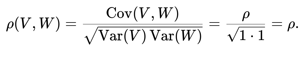
Thus, the vector (V, W) = (X, ρX + √(1−ρ²)Z) has the same mean vector (0,0), identical marginal variances (both 1), and the same correlation ρ as (X, Y). Because it remains a bivariate normal (by construction via linear transformations of a jointly normal pair), it must follow the same distribution as (X, Y).
Representation and Intuition
One intuitive understanding is that for a bivariate normal with correlation ρ, the second variable can always be written as ρX + √(1−ρ²)Z, where Z is independent of X and each has unit variance. This form simply restates that Y is related to X through some scaled version of X plus an independent noise term scaled to achieve the correct marginal variance and correlation.
Practical Example in Python
Below is a short example illustrating how one might simulate this construction to check the empirical distribution:
import numpy as np
import matplotlib.pyplot as plt

# Parameters
rho = 0.7
num_samples = 10_000

# Generate X, Z ~ N(0,1), independent
X = np.random.randn(num_samples)
Z = np.random.randn(num_samples)

# Construct W = rho * X + sqrt(1-rho^2) * Z
W = rho * X + np.sqrt(1 - rho**2) * Z

# Now (X, W) should have correlation rho
empirical_corr = np.corrcoef(X, W)[0,1]
print("Empirical correlation:", empirical_corr)

# Quick scatter plot to visualize
plt.scatter(X, W, alpha=0.2)
plt.title(f"Correlation ~ {empirical_corr:.2f}")
plt.xlabel("X")
plt.ylabel("W")
plt.show()
The empirical correlation of the samples (X, W) will be close to ρ, confirming the theoretical derivation.
Follow-up Question: Why does independence of X and Z ensure W is normal?
Any linear combination of jointly normal random variables is also normal. X and Z are independent normal random variables, which implies that the vector (X,Z) is bivariate normal. Consequently, if you form W as a linear combination ρX + √(1−ρ²)Z, it remains normally distributed. If X and Z were not jointly normal (or not independent), we could not make the same conclusion.
Follow-up Question: What if ρ = ±1?
The condition -1 < ρ < 1 ensures that √(1−ρ²) is strictly positive, so we can construct W = ρX + √(1−ρ²}Z in a non-degenerate way. If ρ = 1 or ρ = -1, the bivariate normal distribution collapses because X and Y are perfectly (or perfectly negatively) correlated. In that case, Y is just ±X without additional noise, leading to a degenerate distribution on a line.
Follow-up Question: How does this generalize to non-zero means or different variances?
If (X, Y) have means mX, mY and variances σX², σY² with correlation ρ, one can standardize to X' = (X - mX)/σX, Y' = (Y - mY)/σY, and similarly introduce an independent standard normal Z. Then Y' could be constructed by ρX' + √(1−ρ²)Z. To recover the original scale, you would scale and shift back: Y = mY + σY[ρ((X - mX)/σX) + √(1−ρ²)Z]. Hence the idea extends naturally to the general bivariate normal case.
Follow-up Question: What are common pitfalls or misunderstandings?
One common pitfall is to assume that any correlation structure can be expressed in terms of a single normal variable plus independent noise. While this works for the 2D (bivariate) case, for higher dimensions one must consider covariance matrices and potentially use tools like the Cholesky decomposition to build random vectors with a specified covariance structure. Another misunderstanding is to overlook that normality of individual coordinates does not guarantee joint normality. One must ensure that every linear combination is normal—hence the importance of starting from an already jointly normal (X, Z).
Below are additional follow-up questions
What if X and Z were merely uncorrelated but not strictly independent?
When we say X and Z are independent and normal, it automatically implies that any linear combination of them is also normal. However, uncorrelatedness alone does not guarantee independence—especially in non-Gaussian settings. If X and Z were merely uncorrelated but had some higher-order dependency structure (e.g., a non-linear relationship), then the vector (X, ρX + √(1−ρ²)Z) would not necessarily be bivariate normal. In fact, for variables that are not Gaussian, uncorrelatedness can coexist with more subtle forms of dependence.
A deeper pitfall arises if one tries to assume that zero correlation is enough to treat them "like independent." This works for Gaussian variables but is not generally valid otherwise. For a proper bivariate normal construction, independence of X and Z is the safest route to ensure that any linear combination remains normally distributed.
How do numerical stability or precision issues arise in practice?
In real-world simulation or sampling scenarios (e.g., Monte Carlo methods), finite-precision arithmetic can lead to slight deviations from the exact correlation ρ. Specifically, if ρ is extremely close to 1 or -1, then √(1−ρ²) becomes extremely small, and floating-point inaccuracies might dominate. This can cause the sampled correlation to deviate noticeably from the target value.
A related edge case arises if ρ is set to exactly 1 or -1 by mistake. Then √(1−ρ²) = 0, making W = ρX + √(1−ρ²)Z become ±X, which destroys any “two-dimensional” nature of the distribution (they collapse onto a line, effectively degenerating). Careful handling of near-unit correlation in real code is essential, often involving checks for boundary conditions or using more numerically stable transformations (e.g., using truncated values of ρ to ensure it is strictly between -1 and 1).
How would we extend this to higher dimensions?
For more than two correlated normal variables, we can generalize this idea by looking at the covariance matrix. Suppose we want a d-dimensional normal vector X with mean vector 0 (for simplicity) and a covariance matrix Σ that is positive semidefinite and symmetric. One standard procedure to generate it is:
Generate a d-dimensional vector of independent standard normals Z.
Compute X = A Z, where A is a matrix such that A A^T = Σ (e.g., a Cholesky factor of Σ).
Each component of X is then a linear combination of the independent standard normals in Z, preserving the normality, but now the covariance structure is controlled by the matrix A. A pitfall is ensuring Σ is valid (i.e., positive semidefinite) and that the numerical factorization (e.g., the Cholesky decomposition) is stable in higher dimensions.
What if we attempt to use ρX + some function f(Z) instead of √(1−ρ²)Z?
One might wonder if ρX + f(Z) could still yield a bivariate normal distribution with correlation ρ, as long as X and Z are independent. However, the shape of the distribution depends on f. To maintain normality, f(Z) must be a linear transformation of Z. If f is nonlinear (e.g., f(Z) = Z² or sin(Z)), the second variable would no longer be a linear combination of normal variables, and the resulting pair would cease to be truly bivariate normal (though it could still have correlation ρ, it would have different higher-order moments).
How is this formula used in regression simulation or synthetic data generation?
When simulating synthetic data with a controlled correlation, especially for testing or benchmarking statistical or machine learning models, one often needs two variables X and Y with a specific correlation. This approach (using X ~ N(0,1), an independent standard normal Z, and defining Y = ρX + √(1−ρ²)Z) is a straightforward and reliable way to generate samples matching the desired correlation. A subtlety arises when scaling to a general correlation matrix across multiple variables or incorporating different marginal distributions.
Moreover, when generating data for regression tests, one might fix the correlation structure among multiple predictors or between predictors and a response variable. The main pitfall is ensuring that the synthetic correlation you design actually matches the real-world correlation structure of the problem you want to emulate. If the real data have skew, heavy tails, or other complexities beyond normality, simply using this bivariate normal approach might misrepresent crucial aspects of the dataset.
How does sampling error impact empirical correlation estimates?
In practical simulations, if you generate n samples of (X, W) and then compute the sample correlation, you will only approximate the theoretical correlation ρ. The sample correlation might differ from ρ by a random amount that shrinks as n grows large. If n is too small or ρ is very close to ±1, numerical issues or sampling variability could cause your empirical correlation to deviate substantially from the theoretical value.
For instance, with extremely high ρ, a small sample might spuriously exhibit slight correlation above 1 or below -1 due to finite-sample noise, causing confusion in some statistical packages. Ensuring sufficiently large sample sizes and verifying approximate normality can help reduce these artifacts.
Are there scenarios where a high-level correlation framework fails?
When dealing with time series or data exhibiting autocorrelation, simply controlling correlation at one time point might fail to capture temporal dependencies. Also, in certain domains (e.g., finance, climate models, or biological measurements), correlations may shift over time or under different conditions, so a single ρ might be too rigid. Another complication arises if the data are heavily non-Gaussian with extreme outliers. Although the formula ρX + √(1−ρ²)Z is mathematically sound under normal assumptions, in real-world heavy-tailed phenomena (e.g., Cauchy distributions or generalized Pareto distributions), correlation alone might not fully encapsulate the dependence structure, and using a Gaussian-based method can be misleading.
What if the marginal distributions of X or Z are not exactly normal?
If X and Z do not both follow normal distributions, then constructing ρX + √(1−ρ²)Z might not yield bivariate normal behavior. For instance, if X is normal but Z is some skewed distribution, the second component will inherit that skew. You would still get a correlation ρ by controlling the linear weights, but the resulting pair won’t be bivariate Gaussian.
In practice, if one needs an approximately Gaussian pair but only has data drawn from a different distribution, a common technique is to apply transformations (like the rank-based inverse normal transform) to create variables that are closer to normal, then apply the correlation structure, and finally transform back to the original space. However, that final transformation generally destroys perfect normality and might alter the correlation in non-trivial ways.