ML Interview Q Series: Convexity Guarantees for Gradient-Based Optimization in Machine Learning Models.

📚 Browse the full ML Interview series here.

Convexity in Optimization: Why is it beneficial if a machine learning optimization problem is convex? Provide an example of a convex loss function used in ML (and the corresponding algorithm). Discuss what guarantees convexity gives for gradient-based optimization.

Heading on Convexity in Optimization

Convexity is an extremely important concept in optimization for machine learning. A function is convex if for any two points in its domain, the line segment connecting these points lies above or on the function’s graph. In other words, whenever we are “between” two points in the input space, the function’s value at that in-between point will not exceed the linear interpolation of the function values at the two endpoints. This structural property simplifies theoretical analysis and facilitates more reliable numerical optimization.

When a machine learning optimization problem is convex, it often means that our loss function (the objective function we want to minimize) is convex with respect to the model’s parameters. This ensures that any local minimum is also a global minimum. By contrast, if the loss function is non-convex, we might get stuck in suboptimal local minima, saddle points, or plateaus, which can complicate both the training dynamics and theoretical guarantees.

Sub-heading on Benefits of Convexity in Machine Learning

Convexity gives strong theoretical guarantees about the optimization process. First, for a strictly convex function, any local minimum is unique and also the global minimum. This uniqueness can be crucial in tasks such as linear regression or logistic regression, where the shape of the loss surface is well-understood.

Convex problems also permit a variety of well-studied optimization algorithms (like gradient descent, coordinate descent, quasi-Newton methods) with proofs of convergence. For example, in convex settings, these algorithms converge to the global optimum under mild conditions. This is a significant advantage because it allows practitioners to predict behavior and performance. Convergence rates and iteration complexities are more readily available in convex optimization theory, giving a clearer picture of how many steps or how much computational effort is needed to reach an acceptable solution.

Sub-heading on Example of a Convex Loss Function

One canonical example of a convex loss function is the logistic loss used in logistic regression. Consider a dataset of input features and binary labels, where each label is either 0 or 1. Let:

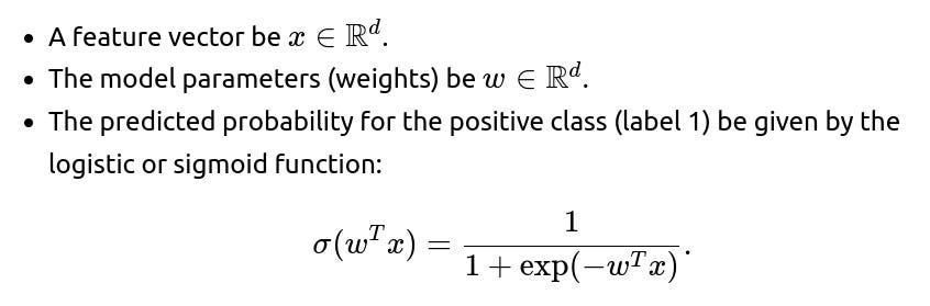
The logistic loss (also called cross-entropy loss for binary classification) for a single data point can be written as:

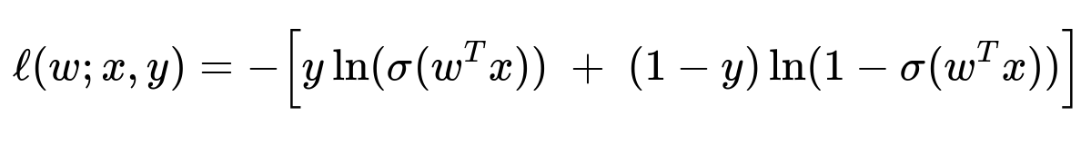
where y∈{0,1}. This loss is convex with respect to w for a fixed feature vector x and label y. Although the logistic function σ(⋅) itself is not linear, the negative log-likelihood form for logistic regression turns out to be a convex function in the parameters.

Corresponding Algorithm: Logistic Regression Training via Gradient-Based Optimization

One straightforward approach to optimize the logistic loss is to use gradient descent or one of its variants (e.g., stochastic gradient descent, mini-batch gradient descent, or advanced methods such as Adam). For logistic regression, each step computes the gradient of the loss with respect to the parameters w and updates w accordingly.

Sub-heading on Guarantees Provided by Convexity

If the loss function is convex, gradient-based methods come with rigorous guarantees:

They do not get trapped in local minima that are suboptimal. Convergence to the global minimum is guaranteed (with mild assumptions on step sizes, etc.). Convex problems often have well-defined strong convexity properties. Strong convexity implies faster convergence rates. For example, if the loss is

-strongly convex, the solution of gradient-based algorithms converges linearly in terms of the distance to the optimum under suitably chosen learning rates. In high-dimensional settings, the convex structure can reduce the complexity of hyperparameter tuning and make the entire pipeline more robust, because the optimization surface does not have complex pathological geometries like saddle points or numerous local minima. Because of these properties, convex methods are especially popular in situations where interpretability, guaranteed convergence, and theoretical clarity are paramount (e.g., some linear models, kernel-based methods like support vector machines with convex hinges, or certain forms of regularized regression).

Heading on Potential Follow-up Questions and Detailed Explanations

What happens if the problem is not convex? Will gradient descent still work?

If the problem is not convex, the loss function might exhibit local minima, saddle points, or flat regions. Gradient descent or its variants can still be used in many non-convex problems (particularly in deep learning), but:

They might converge to a suboptimal local minimum or a saddle point. However, in deep learning practice, surprisingly many local minima can generalize reasonably well, or the landscape might exhibit wide basins that converge to decent solutions. Additional techniques (random restarts, momentum, better learning-rate schedules, or advanced optimizers like Adam or RMSProp) may be needed to avoid being “trapped” in poor regions of the parameter space. But unlike the convex case, there is no global guarantee of optimality.

This means that while gradient-based methods often still work well, we lose the universal guarantee that any local minimum is globally optimal.

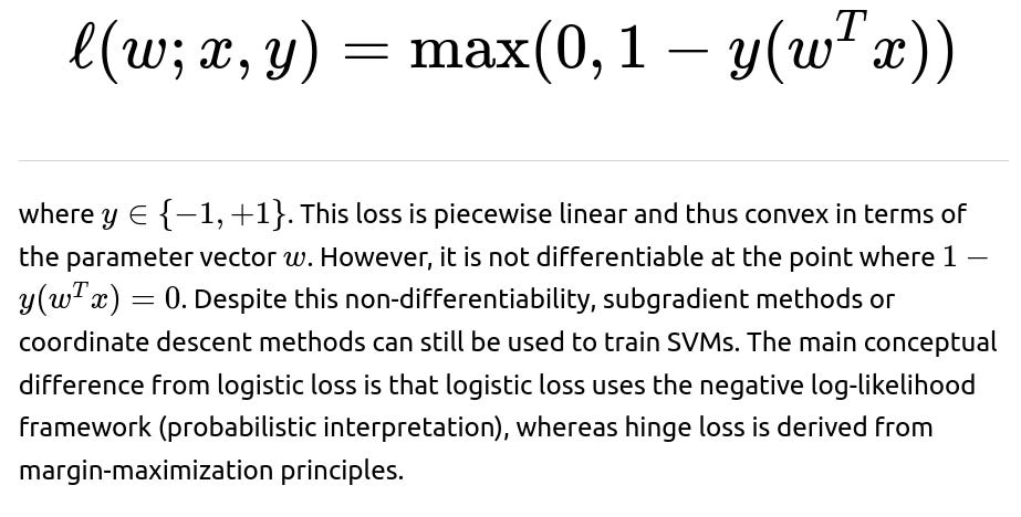
Is the hinge loss for SVMs also convex, and how does it differ from logistic loss?

Yes, the hinge loss used by linear Support Vector Machines is also convex. The hinge loss for a single training example can be written as:

How does regularization interact with convexity?

It helps to reduce overfitting by penalizing large parameter values. It preserves the theoretical optimization guarantees, so the overall objective remains convex, and standard convex optimization approaches still apply.

If the function is strictly convex, what does that imply?

Strict convexity generally implies there is only one unique global minimum. In strict convexity, the function satisfies stronger conditions than ordinary convexity, which often guarantees that the set of solutions to the optimization problem reduces to a single point. This uniqueness is useful when we want to ensure a stable solution to the parameter estimation; for example, different initialization seeds in gradient-based approaches all lead to the same model parameters, ensuring reproducibility.

Can we always use analytical solutions for convex problems?

Not always. Some convex problems, like ordinary least squares linear regression, have closed-form solutions for the optimum. However, many convex problems (e.g., logistic regression or large-scale linear SVMs) do not have neat closed-form solutions. In those cases, we rely on iterative numerical methods like batch gradient descent, stochastic gradient descent, coordinate descent, or quasi-Newton methods (like L-BFGS). These methods still converge to the unique global minimum, but we do not have an expression that directly gives the parameters as in the least squares case.

Does convexity matter for generalization performance or just for optimization?

Convexity primarily simplifies the optimization landscape. It ensures that our search for the minimum is more predictable and that we do not get trapped in suboptimal local minima. However, generalization performance depends on more than just convexity. It depends on:

How well the model architecture matches the problem. The complexity of the feature space or hypothesis class. Regularization methods. The distribution of training data.

Still, a convex model like logistic regression or SVM can be strong baselines or final production models because it is both robust in training and interpretable. But even a convex model can overfit or underfit if the feature representation or regularization is not chosen properly.

Could you provide a short code snippet that illustrates optimizing a convex loss function like logistic loss in Python?

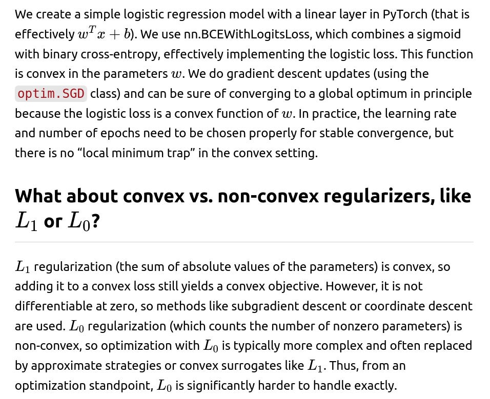
Below is a concise example using PyTorch to perform logistic regression via gradient descent. Although this is a very basic snippet, it captures the essence of convex optimization with logistic loss.

import torch
import torch.nn as nn
import torch.optim as optim

# Example: simple dataset
X_data = torch.randn(100, 5)  # 100 samples, 5 features
y_data = (torch.randn(100) > 0).float()  # binary labels (0 or 1)

# Model definition: logistic regression
model = nn.Linear(5, 1)  # linear layer: input_dim=5, output_dim=1

# Loss function: Binary Cross Entropy with logits
loss_fn = nn.BCEWithLogitsLoss()  # this includes the sigmoid internally

# Optimizer: gradient descent (in practice use Adam or similar)
optimizer = optim.SGD(model.parameters(), lr=0.01)

for epoch in range(1000):
    optimizer.zero_grad()
    logits = model(X_data).squeeze()          # shape [100]
    loss   = loss_fn(logits, y_data)          # scalar
    loss.backward()                           # compute gradients
    optimizer.step()                          # update parameters

# After training, model parameters are near global optimum for this convex problem
print("Trained weights:", model.weight.data)
print("Trained bias:", model.bias.data)

In this snippet:

Are there any real-world pitfalls in applying convex optimization in machine learning?

Although convex problems offer strong theoretical guarantees, real-world issues can occur:

In very high-dimensional settings, direct gradient methods can still converge slowly. Stochastic or mini-batch methods are often used for computational efficiency. The data might be non-linearly separable in its raw form, so transformations or kernel methods might be required. While the kernel trick can preserve convexity for SVMs, it can still become computationally expensive with large data. Regularization terms need to be chosen carefully to balance bias-variance tradeoffs. If the regularization is too strong, underfitting might occur; if too weak, overfitting can happen despite convexity. Feature engineering is critical. A convex method can only do so much if the features are not informative enough.

Because of these constraints, while convex optimization is theoretically elegant and can be computationally efficient for moderately sized problems, very large or extremely complex data might still pose challenges even for convex approaches.

Why do deep neural networks typically use non-convex functions?

Deep neural networks stack multiple non-linear transformations, yielding highly non-convex loss surfaces in the parameter space. This is often beneficial from a representational perspective: the expressive power of neural networks can model complex relationships. But the trade-off is that the optimization becomes non-convex, with no absolute guarantee of finding a global minimum. Practical heuristics, large-scale gradient-based optimizers, careful initialization, and robust training schedules are then used to handle the non-convex nature. Despite the theoretical difficulties, in practice, these heuristics often find good solutions.

Does convexity guarantee the best generalization possible?

Convexity guarantees finding the global minimum of the training loss, but it does not necessarily guarantee the global best in terms of generalizing to unseen data. Overfitting or underfitting can still occur if the chosen model capacity or regularization is not aligned with the true complexity of the task. So convex optimization ensures you solve your training problem optimally, but how well that translates to real-world performance depends on the problem setup, data distribution, feature engineering, and regularization strategy.

Example of a subtle difference between strong convexity and mere convexity in an ML scenario

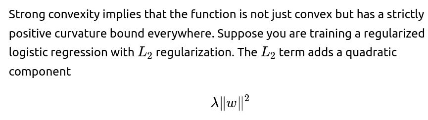
which is strongly convex. This implies faster convergence rates for gradient methods because the curvature of the loss function around the optimum helps “pull” the parameters more strongly to that optimum, reducing the number of iterations required. If the function is only convex but not strongly convex, convergence might still happen, but potentially more slowly.

Such differences can matter a great deal in large-scale machine learning pipelines, where the computational budget and iteration count can be quite large. Having a strongly convex objective can be a practical advantage in designing efficient algorithms.

Can convex optimization approaches handle complex data distributions?

Convex optimization is about the shape of the loss function in parameter space, not the complexity of data distribution per se. Even if the underlying data generation process is complicated, as long as you can represent the hypothesis (model parameters) and define a convex loss with respect to those parameters, the optimization itself is convex. However, you might need feature transformations, kernels, or other techniques to ensure your model can capture the complexities of the data. The success of a convex model in complex domains will hinge on how well the chosen model class (e.g., kernel methods, basis expansions, or carefully engineered features) can fit the data distribution. The optimization remains predictable, but the ultimate predictive power depends on how expressive the model is for the given data.

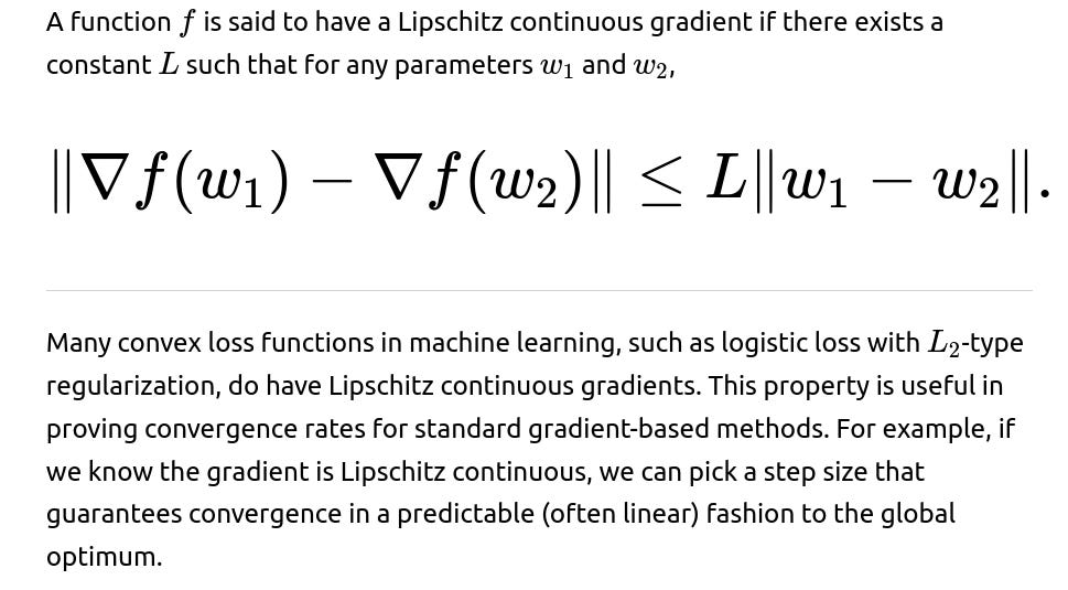
How does the concept of gradient Lipschitz continuity fit with convex problems?

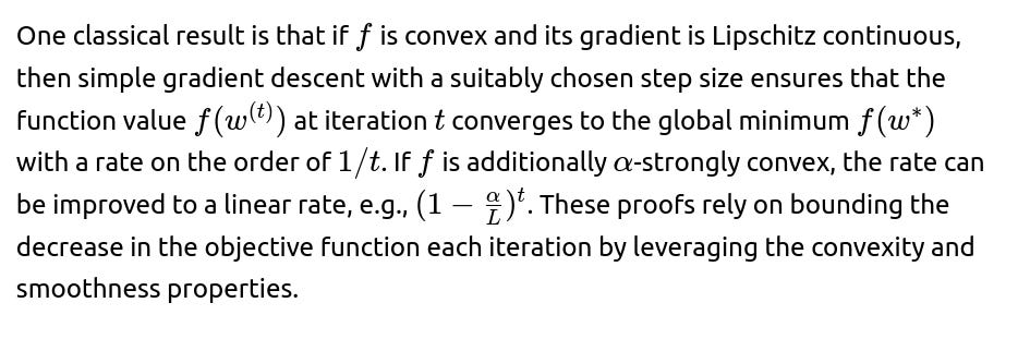
Could you provide a bit more detail on gradient-based proofs of convergence for convex functions?

In practice, does one always see these ideal behaviors with convex functions?

Practical results usually align quite well with theoretical guarantees, though not always perfectly. A few real-world issues can degrade performance:

Numerical stability or precision errors, especially in very large-scale problems. Difficult data distributions can still slow convergence if the features have very large variance or are poorly scaled. Feature scaling (like standardization, min-max normalization) or whitening helps rectify this. Improper step sizes can still cause slow convergence or even divergence. Nevertheless, convex problems remain more predictable than non-convex ones, and in moderate-scale or well-prepared datasets, theory and practice can match closely.

How would you summarize the main takeaway for why convexity is beneficial?

Because convexity ensures that local minima are global minima, training becomes much more straightforward, stable, and theoretically guaranteed to find the best possible solution for the given model class and loss. This drastically reduces the complexity of analyzing, tuning, and applying optimization algorithms. Even though modern deep learning relies heavily on non-convex setups, convex optimization still underpins many classical and interpretable models (like linear/logistic regression, SVMs, many matrix factorization problems, and certain linear matrix completion tasks) and is a core concept for understanding optimization in machine learning.

---

Below are additional follow-up questions

How do approximate solutions or early stopping behave in convex optimization compared to non-convex optimization?

One key property of convex optimization is that we know the global optimum is unique or at least that any local minimum is also global. In many practical scenarios, however, we do not always run the optimization until complete convergence. We might use early stopping to reduce computational expense or to avoid overfitting. In convex settings, when we stop early, we can still be confident that if we continued with small, well-chosen steps, we would eventually converge to the global minimum. Early-stopped solutions in convex problems also tend to be easier to analyze theoretically; we have bounds on how the objective differs from the global optimum if we know the learning rate and number of iterations.

In contrast, for non-convex optimization (like neural networks), early stopping might land us in a local minimum or a plateau. Sometimes, ironically, these local minima or wide basins can yield decent generalization. But there is no universal guarantee that moving further would not yield a better solution. That uncertainty does not arise in convex problems, where “further exploration” eventually leads to the global solution.

In terms of pitfalls, if the learning rate is poorly tuned even in a convex setting, we might see a very slow convergence or oscillations. Early stopping under those circumstances can produce a suboptimal parameter set, even though in principle the objective is nice and convex. Another subtlety is that for large-scale data, even in convex scenarios, one might rely on mini-batch updates that introduce noise. Convergence in such stochastic settings is typically proven under assumptions about the diminishing learning rate or batch sizes growing over time; failing to tune these carefully can undermine the advantages of convexity.

What is the role of second-order methods (Newton’s method) in convex optimization, and how do they compare to first-order methods?

Second-order methods leverage curvature information (i.e., the Hessian matrix of second derivatives) to take more informed steps during optimization. In strictly convex problems, Newton’s method can converge very quickly, often quadratically near the optimum. That means that once you are in the neighborhood of the global minimum, you reduce the distance to the optimum at an extremely fast rate each iteration.

However, second-order methods carry higher per-iteration costs because computing and inverting (or approximating the inverse of) the Hessian can be expensive, especially for large-scale problems with high-dimensional parameter spaces. This computational burden sometimes outweighs the theoretical convergence benefits. As a result, in many modern machine learning tasks (even convex ones), practitioners often use first-order or quasi-Newton methods (like L-BFGS) that approximate Hessian-vector products without storing the full Hessian.

A subtlety arises if the Hessian is nearly singular or if the condition number (the ratio of largest to smallest eigenvalues) is very large. In that case, naive Newton updates might not be stable or might require specialized regularization of the Hessian. This can lead to numerical instabilities if not handled properly. Still, in well-conditioned convex problems with moderate dimension, second-order methods can outperform simpler approaches in terms of number of iterations to convergence.

What if the convex loss function is subject to additional constraints, such as parameter bounds or domain restrictions?

Constraints in convex optimization can be handled by techniques such as projected gradient descent, proximal methods, or the method of Lagrange multipliers (when the constraints are themselves convex sets). For example, if you have a parameter vector that must remain within a box constraint or a simplex (as in certain probability or portfolio allocation problems), you can project your updated parameters back into the feasible region after each gradient step. Because both the loss and the constraint set are convex, the overall problem remains convex, preserving guarantees of a global optimum.

Are there scenarios where a function is convex in only a subset of directions or a subset of parameters, and how does that affect training?

Functions can be partially convex or “convex in blocks.” For instance, in matrix factorization, you might have a function that is convex in one factor matrix if the other is held fixed, but not convex jointly in all parameters. This is sometimes referred to as biconvex or multiconvex structure. A biconvex function is not truly convex in the entire parameter space simultaneously; however, if you treat one set of parameters as fixed, then the function in the other parameters might be convex. This is the basis for alternating minimization methods (where you optimize w.r.t. one block of parameters at a time).

The pitfall is that although each sub-problem is convex, the overall problem can be non-convex. This means that the guarantee of a global minimum across all parameters does not hold. You could arrive at a local minimum that is globally optimal for one block but not for the entire parameter set. In practice, alternating minimization can still work quite well, but one must be aware that partial convexity does not bestow the same universal guarantees as true convexity does.

What is the difference between a convex function and a convex set, and why does that matter in optimization?

A convex set is a set where any line segment connecting two points in the set remains entirely within that set. A convex function is a function for which every chord of its graph lies above or on the function. These two notions interact in convex optimization problems that often read: minimize a convex function over a convex set. The feasibility region (where parameters are allowed to lie) is typically taken to be a convex set, ensuring that if you take a convex combination of any two feasible solutions, you stay within the feasible region.

If the feasible set is non-convex, even if the objective function is convex on the entire space, restricting it to a non-convex domain can produce multiple local minima within that domain. This can forfeit the global optimality guarantee. Hence, we need both a convex objective and a convex feasible set (or no constraints at all) to exploit the full power of convex optimization.

Can certain non-convex problems be turned into convex ones through transformations or special reparameterizations?

Yes, sometimes a carefully chosen reparameterization or transformation can make a non-convex problem convex. A classic example is if you have a problem where the variable is restricted to be positive, and you perform a log transformation to turn a multiplicative constraint into an additive one, potentially converting a non-convex constraint or objective into a convex one in the new domain. Another example arises in logistic regression with certain monotonic link functions: if the structure is properly set up, the effective problem in parameter space can remain convex, even though the raw formulation might look non-linear.

However, such transformations do not always exist or can be complicated to derive. Sometimes the transformation might solve convexity but introduce other complications: the domain might shift, or the transformation might cause numerical instabilities (for instance, log(0) is undefined if you ever get zero-valued variables). Additionally, even if the function becomes convex, it might be much harder to handle in practice due to ill-conditioned transforms or large curvature changes.

How do we handle very large-scale convex optimization problems in distributed or parallel computing environments?

In large-scale or distributed setups, one might employ techniques like mini-batch stochastic gradient descent (SGD), coordinate descent, or asynchronous parallel algorithms. The advantage in convex settings is that each partial gradient step taken (even if computed on a subset of data or run asynchronously) still progresses overall toward the global minimum. There are theoretical guarantees that if each worker applies updates consistently and the learning rates are controlled, the overall method converges to a global optimum.

The pitfall is that in distributed environments, delays or partial parameter updates can cause stale gradients. For instance, one worker might be computing a gradient based on outdated parameters if communication is lagging. While convergence is still guaranteed in many convex setups, the convergence rate might degrade or require more careful synchronization and learning-rate tuning. Another subtle issue is memory constraints: a naive second-order method is often infeasible for extremely large parameter spaces. That is why large-scale linear models typically rely on (stochastic) first-order updates.

How can outliers or noisy data distributions affect the performance of convex optimization methods?

Most convex losses, such as the squared error in linear regression, can be sensitive to outliers because the function grows quadratically with large residuals. Even though the optimization is convex, a small number of extreme data points might disproportionately influence the solution. Logistic loss is slightly more robust than squared loss in classification contexts, but it can still suffer if the data are extremely noisy or mislabeled.

In real-world scenarios, one might mitigate outlier sensitivity by choosing a robust loss function (e.g., Huber loss, which is convex but less sensitive to large residuals than the squared loss) or by applying data cleaning procedures. A less robust approach might still converge to the global optimum of the chosen loss, but that optimum might not be desirable from a modeling standpoint if it has been heavily skewed by a few erroneous data points.

Are there strictly convex ML tasks that are still hard in practice due to resource limitations?

Yes, some ML tasks are strictly convex yet involve enormous datasets or extremely high-dimensional feature spaces, making them computationally challenging. For example, a large-scale ridge regression with billions of features is strictly convex but may be prohibitively expensive to solve with naive algorithms. In such cases, practitioners resort to:

Stochastic or mini-batch approaches that scale to large data. Sparse or approximate methods that reduce computational overhead. Dimensionality reduction or feature screening that lowers the effective dimensionality before solving the convex problem.

The pitfall is that while the objective remains convex, approximations or partial solutions might degrade the final accuracy. Still, the advantage is that even approximate solutions in strictly convex problems often come with explicit bounds or well-understood trade-offs. For instance, random feature maps for kernel methods preserve enough of the kernel’s structure to yield near-optimal solutions with lower computation than a full kernel matrix, retaining the convex property but on a reduced representation.

Do we need multiple initializations in convex problems, and can random starts help anyway?

For a purely convex objective with no constraints that break convexity, multiple initializations should, in theory, converge to the same global minimum. This is because there are no suboptimal local minima to escape from. Practitioners typically do not need random restarts in such scenarios since a single run of gradient descent or another suitable method will find the global optimum regardless of where it starts.

However, random initializations might still provide advantages in special circumstances. If you have partial convexity, constraints creating non-convex feasible sets, or approximate numeric methods that can behave unpredictably in certain regions (like heavy regularization with non-differentiable points), different starts might converge more reliably or more quickly. In strictly convex settings without complicated constraints, though, random restarts generally end up at the same solution, so they do not provide an additional benefit in terms of escaping local minima. They might, however, provide minor benefits in terms of faster route to convergence if some starting points are exceptionally well aligned with the gradient. But typically, well-chosen initialization or standardized data features ensure that one start suffices.