ML Interview Q Series: Could you compare the pros and cons of different classification algorithms, and how would you select the most suitable one in practice?

📚 Browse the full ML Interview series here.

Comprehensive Explanation

Classification algorithms vary in terms of their expressiveness, training complexity, interpretability, computational requirements, and robustness to noisy data. Factors like the size of your dataset, data dimensionality, the presence of outliers, and the need for interpretability can all influence which classifier works best in a given scenario. Some algorithms have a faster training speed but might be less flexible in decision boundaries, whereas others might capture complex relationships in the data but at the cost of interpretability or computational cost.

Trade-Offs and Characteristics of Common Classification Algorithms

Logistic Regression

This method is widely used for binary classification and is favored for its interpretability. It models the probability of a class using the logistic (sigmoid) function applied to a linear combination of input features. One way to express the predicted value is:

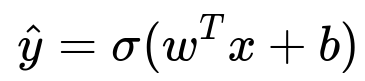
Where the parameter vector w and the scalar b represent the model’s coefficients and intercept. The symbol x denotes the input features. The function sigma(z) = 1 / (1 + e^-z) squashes any real input into the (0,1) range.

Logistic Regression tends to perform well when there is a linear decision boundary between classes. Its coefficients are highly interpretable as each weight corresponds to how strongly a feature contributes to the probability of belonging to a particular class. However, if your dataset has complex or non-linear decision boundaries, Logistic Regression might underfit unless you create polynomial or non-linear feature transformations.

Support Vector Machines (SVM)

SVMs create a decision boundary (or hyperplane) that maximizes the margin between different classes. They can use the kernel trick to handle non-linear relationships by mapping data into higher-dimensional feature spaces. This often makes SVMs very powerful when your data is not linearly separable in the original input space.

They can be quite memory-intensive for large datasets, particularly with complex kernel functions. Also, choosing the right kernel and tuning parameters such as the regularization parameter and kernel-specific parameters (like the RBF kernel width) can be challenging.

Decision Trees

Decision Trees partition the data space into regions based on the features’ values. They are very intuitive and interpretable because you can follow the path from the root to a leaf node to determine how a prediction is made. Trees can capture non-linear relationships and interactions among variables without manual feature engineering.

They tend to overfit easily, especially deep trees that keep splitting until each leaf has very few instances. Pruning and other techniques help mitigate overfitting. Also, small changes in the training set can drastically alter the structure of the tree.

Random Forests

Random Forests are an ensemble of Decision Trees where each tree is trained on a bootstrap sample of the data, and a subset of features is randomly selected at each split. The final prediction is typically determined by majority vote (for classification tasks). Because the model averages over many different Decision Trees, Random Forests tend to have high predictive power and reduce the variance inherent in single Decision Trees.

Random Forests can handle large feature spaces well and are robust to noise. However, they can be less interpretable as an ensemble because it’s more difficult to understand the exact reasoning from hundreds of trees.

Gradient Boosting Machines (XGBoost, LightGBM, CatBoost)

These methods train ensembles of weak learners (often small Decision Trees) in a stage-wise fashion. Each new tree attempts to correct the errors of the previous ones. Models like XGBoost often achieve state-of-the-art results in many structured data tasks, due to their ability to capture complex patterns and reduce bias and variance effectively.

They are sensitive to hyperparameters like the learning rate, number of estimators, and tree depth. Tuning them can be time-consuming, but when done properly, they often outperform simpler methods on tabular datasets.

k-Nearest Neighbors (k-NN)

k-NN is a simple, instance-based learning approach that does not require explicit training. Classification is done by a majority vote of the nearest neighbors in the feature space. Choosing the right distance metric and the value of k is crucial. As k-NN relies on comparing a test instance to all training samples, it can become computationally expensive for large datasets. It also doesn’t produce an explicit model, which can make interpreting results challenging.

Neural Networks

Neural Networks, particularly Deep Neural Networks, can model extremely complex relationships in data when provided with enough training examples. They can automatically discover underlying structures in high-dimensional data. However, they require significant computational resources, can be prone to overfitting if not regularized, and typically have large numbers of hyperparameters. They are also less interpretable, though methods like feature visualization and sensitivity analysis can partially address this.

Choosing the Best Algorithm

Data Size and Dimensionality Small datasets might favor simpler models like Logistic Regression, SVM with linear kernel, or small Decision Trees to avoid overfitting. Large datasets enable more complex models such as ensembles or Deep Neural Networks to shine.

Interpretability Requirements Models like Logistic Regression and single Decision Trees are straightforward to interpret. Random Forests, Gradient Boosted Machines, and Neural Networks are often more challenging to interpret, though you can use feature importance or SHAP values to glean insights.

Computational Efficiency If training time is critical, simpler methods like Logistic Regression or Linear SVM are usually faster to train. More complex models like ensembles or Neural Networks could be computationally expensive, especially with large datasets.

Model Complexity and Capacity High-capacity models (Neural Networks, large ensembles) can capture complex patterns but risk overfitting. If your data exhibits non-linearities, simpler linear models might not suffice without feature engineering.

Potential Follow-Up Questions

How do you handle imbalanced datasets when choosing a classification algorithm?

Imbalance in classes can seriously impact the performance of most algorithms. Approaches include undersampling the majority class, oversampling the minority class, and generating synthetic samples (e.g., SMOTE). You might also use modified metrics like precision, recall, F1-score, or AUC to get a better measure of performance. Certain classifiers can handle imbalance inherently by adjusting class weights, such as SVM or Logistic Regression with class_weight parameters. Ensemble methods like Random Forests or Gradient Boosting can also incorporate class weights to focus on the minority class.

What if you have very high-dimensional data?

When the number of features is much larger than the number of samples, you should consider dimensionality reduction or regularization. Methods like PCA or autoencoders (for Neural Networks) can help reduce noise in very high-dimensional data. Regularized models like L1-regularized Logistic Regression or SVM can also be effective. In extremely high-dimensional scenarios, using simpler linear classifiers with strong regularization often provides a robust baseline.

How do you balance interpretability versus accuracy?

In many domains, especially regulated industries, interpretability is crucial. You might opt for simpler algorithms like Logistic Regression or small Decision Trees so domain experts can understand how decisions are reached. If accuracy is paramount and interpretability is less critical, ensembles or Neural Networks might be acceptable. In some cases, you can deploy a complex model for raw predictive power while also training a simpler interpretable model to approximate the predictions.

Is there a systematic procedure to select the model?

A common strategy is to start with simple baseline models (Logistic Regression, Decision Trees) to gain insights into the problem, dataset, and relevant features. Evaluate performance using cross-validation and metrics that match your business objectives. You can then iterate to more advanced models (Random Forest, Gradient Boosting, Neural Networks) if you see potential gains. Model selection ideally involves both quantitative comparison (accuracy, precision, recall, F1, etc.) and practical considerations (interpretability, computational cost, ease of deployment).

What common pitfalls might you face with classification?

You might overfit if you choose overly complex models or do excessive hyperparameter tuning without regularization. You might also underfit with overly simple models or if you do not capture the true non-linearities in the data. Class imbalance can lead to misleading accuracy metrics. Data leakage occurs when features contain information about the target in ways that would not be available in practice. Failing to do proper cross-validation can lead to overly optimistic estimates of model performance.

You can address these pitfalls by doing thorough data exploration, applying cross-validation, carefully tuning hyperparameters, and checking for leakage in the features.

Below are additional follow-up questions

Could you elaborate on the difference between generative and discriminative classifiers, and how these distinctions impact real-world usage?

Generative classifiers (like Naive Bayes, Gaussian Mixture Models) attempt to learn the joint probability of features and labels. From that joint distribution, they derive posterior probabilities to classify new data points. By contrast, discriminative classifiers (like Logistic Regression, SVM) directly learn the decision boundary or conditional probability of labels given features without explicitly modeling how the data is generated.

Generative models can be advantageous when you have limited training data or when you need to model missing data scenarios, because they capture the underlying distribution of your features. They can also be used for data generation, anomaly detection, or semi-supervised setups. However, if the model’s assumptions about the data distribution (e.g., independence of features in Naive Bayes) are violated, performance could degrade. Another potential drawback is that fully specifying the joint distribution in high-dimensional spaces can be complex and prone to error if the assumed distribution is not a good fit.

Discriminative models tend to be more flexible in capturing complex decision boundaries and often deliver higher predictive accuracy in practice if sufficient labeled training data is available. On the flip side, they do not provide insight into the way the data was generated. If you want interpretability in a probabilistic sense or need to handle missing features at inference time, you might find pure discriminative methods less amenable compared to a generative approach.

Real-world issues arise when data distributions shift or contain outliers that violate the assumptions of a generative model. Generative classifiers can become miscalibrated quickly if the underlying distribution changes unexpectedly. Discriminative methods may cope better with slight changes to the feature distributions, but they might also become brittle if the shift introduces significantly new patterns not captured in training.

What methods can be used to deal with concept drift in classification tasks, and what pitfalls might arise?

Concept drift refers to changes in the statistical properties of the target variable or features over time. This is common in scenarios like streaming data, user preferences, or evolving sensor readings. Common ways to address concept drift include online learning methods that update the model incrementally, periodic retraining of batch models on recent data, or using ensemble techniques that weight recent models more heavily.

A potential pitfall is forgetting older but still relevant patterns if the data reverts to a previous state later. In abrupt drift, the distribution changes quickly, which can render a model’s prior knowledge useless unless it’s adapted rapidly. However, if the model is tuned too aggressively to short-term changes (for example, retraining too frequently or giving too much weight to recent data), it might degrade performance when patterns revert. Another subtlety is distinguishing between true concept drift and noise. High variability could be mistaken for concept drift, leading to unnecessary updates that increase model instability.

How do you handle missing or incomplete data in classification, and what considerations drive the choice of method?

Handling missing data often involves imputation techniques or modeling strategies that are robust to incomplete feature sets. Common imputation techniques include mean/median filling for continuous variables or mode filling for categorical variables. More sophisticated methods use regression or model-based imputation (e.g., k-NN imputation, MICE).

One pitfall is that naive imputation can introduce bias. For instance, using mean imputation for a highly skewed distribution might obscure important signals and artificially reduce variance. Another risk is ignoring the fact that data might be missing not at random (MNAR). In such cases, the reason data is missing carries valuable information, and discarding or blindly filling the entries loses that signal. Additionally, if too many features are missing for each observation, you may need a strategy like building multiple specialized models or applying dimensionality reduction.

The choice of method also depends on the volume and pattern of missingness. If very few samples have missing values, dropping them may be simpler. In high-stakes domains (like healthcare), more careful data analysis is necessary to ensure that patterns of missingness are well understood and accounted for, possibly requiring domain-specific knowledge to avoid systemic biases in how data is filled or removed.

Can you discuss incremental or online learning in classification and highlight subtle pitfalls?

Incremental learning (or online learning) updates the model as new data arrives, rather than training from scratch. Algorithms like Stochastic Gradient Descent (SGD) for linear models, online variants of Naive Bayes, or incremental ensemble methods (like Hoeffding trees) are used in streaming contexts.

One key pitfall is catastrophic forgetting: the model may heavily adjust to recent examples at the expense of performance on previously learned patterns. Striking a balance is tricky—especially if older data can still appear, or if the dataset is cyclical, as is the case with seasonal consumer behaviors.

Another potential trap is the assumption that the input distribution is stationary. If the distribution shifts completely (concept drift), online updates that assume stationarity may significantly degrade model performance. Moreover, hyperparameters (like learning rate) need careful tuning to avoid over-adapting or under-adapting to new data. Ensuring proper memory management is also critical since storing too many historical data points can undermine the advantage of an online approach.

How do domain adaptation or transfer learning methods help when training and test distributions differ, and what tricky issues arise?

Domain adaptation attempts to leverage knowledge gained in one domain (source) and apply it to a different but related domain (target). Common strategies include distribution matching, instance reweighting (e.g., giving more weight to source instances that resemble the target domain), or learning domain-invariant feature representations.

A subtle pitfall is assuming that the source and target domains share a strong underlying structure. In reality, differences in how features are measured or labeled could violate those assumptions. If the target data is extremely sparse or unlabeled, aligning distributions might rely on heuristic measures of similarity that do not capture deeper domain-specific nuances. Also, domain adaptation may fail if certain classes appear in the target domain that never appeared in the source domain.

Transfer learning using pretrained Neural Network models can be powerful, but the initial pretrained model might contain biases from its original training data. These biases can translate to suboptimal or even harmful predictions in the new domain if not carefully fine-tuned. Finally, the process of fine-tuning can overfit if the target domain dataset is small or not representative.

How do you manage multi-label classification in real-world applications, and what uncommon pitfalls might appear?

In multi-label classification, each instance can be associated with multiple labels simultaneously, as opposed to multi-class classification where each instance has exactly one label. Methods include binary relevance (treat each label as a separate binary classification), classifier chains (where predictions of previous labels feed into the next classifier), and more complex algorithms that directly model label dependencies.

One pitfall is ignoring correlations among labels. Binary relevance methods treat labels independently, which can be suboptimal if certain labels almost always co-occur. On the other hand, classifier chains or structured prediction methods can capture dependencies but become more computationally intensive and harder to tune.

Another pitfall is evaluation. Common classification metrics like accuracy become less informative when an instance can have multiple correct labels. Metrics like the Hamming loss, subset accuracy, or F1-based measures for each label can give different perspectives. Furthermore, certain classes in the label set might be very rare, magnifying imbalance challenges.

Are there scenarios where classification evaluation metrics like F1-score, recall, or precision are insufficient, and what alternative metrics might be more appropriate?

In highly imbalanced or specialized tasks, F1-score, recall, and precision might not fully capture the decision-making needs. For example, in credit card fraud detection, the cost of a false negative (missing a fraudulent transaction) is drastically different from the cost of a false positive (flagging a legitimate transaction as fraud). In such cases, cost-sensitive metrics or cost matrices that weigh different error types differently are used to guide model optimization.

Another scenario is when you want to rank predictions, or you care about how well the model discriminates across the entire distribution of predicted probabilities. Metrics like ROC AUC and PR AUC can be more informative than a single precision/recall/F1 value. Yet one subtlety is that PR AUC might be more insightful than ROC AUC for extremely imbalanced data, because ROC AUC can be misleadingly high when negative examples dominate the dataset.

Sometimes business-specific Key Performance Indicators (KPIs) might not match standard metrics. For instance, you might care about the top 100 highest-probability fraud cases for immediate review. In such a scenario, focusing on metrics like precision at k or cumulative gains can be more relevant than standard classification metrics.

How does time-series classification differ from standard classification, and what are the main pitfalls?

Time-series classification involves sequences of observations indexed by time. Unlike standard classification, time-series data may have temporal autocorrelation, seasonality, and trends. Splitting data into training and test sets requires techniques that preserve the temporal order to avoid data leakage (for example, using a random split can inadvertently train on future data). Sliding window or walk-forward validation methods help simulate real-world performance over time.

A major pitfall is ignoring the inherent temporal dependencies. Treating each timestamp as an independent instance can lead to overconfidence if the model inadvertently learns from future points. Feature engineering can also be more complex—capturing lags, rolling means, or other time-dependent attributes. Another subtlety is concept drift over time: the patterns in a time series may shift seasonally or due to events like policy changes. So, a model that performs well historically may degrade quickly if future behavior differs significantly from past trends.

How do correlated features or multicollinearity affect classification models, and what measures can be taken to mitigate it?

When features are highly correlated, models that rely on independent assumptions (e.g., Naive Bayes) can produce biased estimates. Linear models (e.g., Logistic Regression) can have unstable coefficients if features are nearly collinear, which leads to inflated variance in parameter estimates. This instability might cause small data perturbations to produce large swings in predicted outcomes.

Regularization methods (like L2 regularization) mitigate some of these issues by shrinking the coefficients, thus reducing the impact of collinearity. Dimensionality reduction (like PCA) can also help, transforming correlated features into orthogonal components. In Decision Tree–based methods, correlation among features typically means the tree can split on either correlated feature interchangeably, although it rarely leads to as much instability as in linear models. However, it can mask the importance of features that are strongly correlated, because once one correlated feature is chosen, the other might appear less relevant.

What is model calibration, and how might calibration differ across classification algorithms?

Model calibration refers to aligning a classifier’s predicted probabilities with the true likelihood of an event. For example, if your model assigns a probability of 0.7 to some instance, you would ideally want the event to occur about 70% of the time for all instances predicted at 0.7. Platt scaling and isotonic regression are common calibration approaches.

Some algorithms, like Logistic Regression, are inherently better calibrated—Logistic Regression outputs represent probabilities in a direct way (assuming the model is well-regularized and the data meets logistic assumptions). Others, like SVMs, produce decision functions that are not probabilities by default. You might need an additional calibration step (like Platt scaling) to convert decision function values into probability estimates. Tree-based methods like Random Forests or Gradient Boosted Trees can also be poorly calibrated out of the box if they overfit, requiring post-training techniques like temperature scaling or isotonic regression. A subtlety is that if your model is under strong regularization or the data is noisy, calibration can overfit if not carefully validated, especially if you have limited calibration data.