
ML Interview Q Series: Could you describe the essence and purpose of a confusion matrix used in classification tasks?

📚 Browse the full ML Interview series here.
Comprehensive Explanation
A confusion matrix is a tabular representation of the performance of a classification model. In a binary classification setting, it is typically a 2 x 2 table that compares the actual labels against the predicted labels, capturing how many predictions fall into each correct or incorrect category. More formally:
True Positive (TP)refers to the instances where the model predicted positive and the actual label was indeed positive.False Positive (FP)corresponds to the model predicting positive while the actual label was negative (also known as a Type I error).True Negative (TN)indicates the model predicted negative and the actual label was negative.False Negative (FN)is the model predicting negative while the actual label was actually positive (also known as a Type II error).
In practice, a confusion matrix helps visualize the ways in which a classification model may be confusing one class with another. By looking at it, you can spot if there is a systematic bias toward predicting certain classes, or if the model fails to capture particular patterns, leading to incorrect predictions.
When extended to multi-class classification, the confusion matrix grows into an n x n table (where n is the number of classes), with each row representing the true class and each column representing the predicted class.
Below is an example in Python demonstrating how to compute a confusion matrix using scikit-learn:
import numpy as np
from sklearn.metrics import confusion_matrix

# Example ground truth labels and predictions
y_true = [1, 0, 1, 1, 0, 0, 1]
y_pred = [1, 0, 0, 1, 0, 1, 1]

cm = confusion_matrix(y_true, y_pred)
print(cm)
Interpreting the resulting matrix:
The diagonal elements show the count of correct predictions for each class.
Off-diagonal elements reveal class misclassifications.
Beyond mere interpretation, a confusion matrix provides building blocks for common classification metrics such as Accuracy, Precision, Recall, and F1 Score, all of which are essential in understanding model performance.
Accuracy, Precision, Recall, and F1 Score
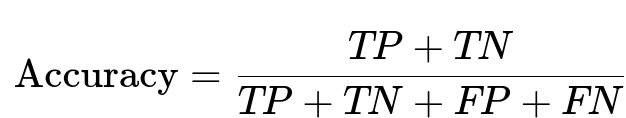
Accuracy calculates how often the model makes the correct prediction, and is given by the ratio of correct predictions (TP + TN) to the total number of predictions (TP + TN + FP + FN).
Where:
TP + TN is the total number of correct predictions (positives correctly labeled as positive plus negatives correctly labeled as negative).
FP + FN is the total number of incorrect predictions.
Precision is the ratio of correctly predicted positive observations (TP) to the total predicted positives (TP + FP). It answers the question: "Of all instances predicted positive, how many are actually positive?"
Recall (also called Sensitivity) is the ratio of correctly predicted positive observations (TP) to all actual positives (TP + FN). It answers the question: "Of all instances that are truly positive, how many did we catch?"

F1 Score is the harmonic mean of Precision and Recall. It combines both measures in a single metric:

In many real-world applications, especially those involving imbalanced data, using only Accuracy can be misleading, and metrics like Precision, Recall, and F1 Score (derived from the confusion matrix) provide more insight.
How do you handle multiclass classification with a confusion matrix?
When dealing with multiple classes, the confusion matrix expands to an n x n matrix, where each row represents one of the n true classes, and each column represents one of the n predicted classes. Each cell (i, j) in the matrix indicates how frequently class i has been misclassified as class j. The diagonal cells still represent correct predictions for each class. One can then compute Precision, Recall, and F1 Score for each class independently and potentially average them (using micro, macro, or weighted averaging schemes) to get an overall sense of how well the model performs across all classes.
In practice, using scikit-learn, this is done automatically when calling confusion_matrix with multi-class labels. The principle remains the same, but analyzing an n x n matrix visually can be more challenging, requiring heatmaps or other visualization techniques.
Why might a confusion matrix be particularly useful for imbalanced datasets?
In highly imbalanced datasets, many instances belong to one dominant class and only a few belong to the minority class. In such scenarios, a simple metric like Accuracy can be deceptive. For instance, predicting every instance as the majority class could yield a high Accuracy score but fail to capture the minority class altogether. The confusion matrix makes it easier to see the actual breakdown of where the model succeeds and fails. Specifically, examining FP and FN becomes critical when dealing with rare but important classes (for example, fraud detection or disease prediction). Observing how many positive examples are missed (FN) or how many negative examples are incorrectly labeled as positive (FP) is crucial to model evaluation.
What are potential pitfalls when interpreting a confusion matrix?
One pitfall is focusing on the absolute numbers without considering the context or class distribution. Another is assuming that a single metric (such as Accuracy) derived from the matrix is sufficient—this could be misleading if there is severe class imbalance. Additionally, confusion matrices can become unwieldy and harder to interpret for a large number of classes (e.g., in a 50-class problem), making it difficult to glean overall performance at a glance. Lastly, one should be aware of the thresholds used to convert model outputs (like probabilities) into predicted classes; different thresholds can produce different confusion matrices and thus different metrics.
How do you choose between different thresholds to improve confusion matrix-based metrics?
Many models (especially those providing probabilistic outputs) allow you to adjust the decision threshold. For example, a default threshold of 0.5 might lead to certain levels of Precision and Recall, but lowering the threshold can catch more positives (increasing Recall) while potentially increasing False Positives. Conversely, raising the threshold might lead to fewer False Positives but also fewer True Positives, hence lowering Recall. Thus, one might plot the Precision-Recall curve or the ROC curve (True Positive Rate vs. False Positive Rate) to select an optimal threshold that balances trade-offs in alignment with the business or application needs.
Is there a common way to visualize a confusion matrix?
A confusion matrix is often displayed as a heatmap, where each cell is color-coded to quickly convey how many instances are in that cell. Such a heatmap can be created using Python libraries like matplotlib or seaborn:
import seaborn as sns
import matplotlib.pyplot as plt
from sklearn.metrics import confusion_matrix

y_true = [1, 0, 1, 1, 0, 0, 1]
y_pred = [1, 0, 0, 1, 0, 1, 1]

cm = confusion_matrix(y_true, y_pred)

plt.figure(figsize=(5,4))
sns.heatmap(cm, annot=True, fmt="d", cmap="Blues")
plt.ylabel("Actual")
plt.xlabel("Predicted")
plt.show()
By labeling rows as actual classes and columns as predicted classes, the heatmap clearly displays where the model predictions are accurate (the diagonal) and where they go wrong (the off-diagonal cells).
Can confusion matrices be used when performing cross-validation?
Yes. You can compute a confusion matrix for each fold in cross-validation, then sum or average them to see how performance varies across folds. This gives a more robust sense of how the model generalizes. However, care must be taken in interpreting these aggregated matrices, because combining them might lose some information about each fold’s idiosyncrasies. It is still often helpful to examine the confusion matrix fold by fold, in addition to looking at the aggregate version.
Could a confusion matrix be used to select hyperparameters?
You can absolutely consider confusion matrix-derived metrics (Precision, Recall, F1 Score) for hyperparameter tuning. For instance, if you care more about minimizing False Negatives than False Positives, you can optimize for high Recall. This can be done via grid search or Bayesian optimization, using the relevant score (such as Recall) as your optimization metric. Observing the confusion matrix after each hyperparameter combination helps ensure that the results reflect meaningful improvements in classification behavior rather than superficial gains in overall Accuracy.
Below are additional follow-up questions
How can cost-sensitive learning be combined with confusion matrices to address misclassifications that have different penalties?
When certain errors are more expensive than others (for example, missing a fraudulent transaction is more costly than flagging a valid one), cost-sensitive learning can help. In such a scenario, you can assign different costs to different types of misclassifications. Here is how a confusion matrix plays a role:
The confusion matrix still shows you counts for True Positives, False Positives, True Negatives, and False Negatives, but now each cell can be associated with a specific cost. For instance, you might have a cost of
5for False Negatives but only1for False Positives, depending on the domain.Instead of aiming purely for overall accuracy, you aim to minimize a total cost function that sums all misclassification costs. For example, a cost function might be: (FP * cost_FP) + (FN * cost_FN) + (TP * cost_TP) + (TN * cost_TN).
You can tune model parameters to optimize this cost function. This might involve threshold tuning or using specialized algorithms (like weighted SVMs or cost-sensitive decision trees).
One subtle pitfall is deciding how to set these costs appropriately. An incorrect or arbitrary cost assignment can lead to suboptimal model behavior. Another is that real-world costs can sometimes be complex or non-static, meaning they shift over time and require repeated recalibration.
Edge cases might include changing costs after deployment, when new information about the severity of errors emerges or when class distributions shift, making it crucial to continuously monitor performance and costs.
What unique challenges arise when using a confusion matrix with noisy or partially labeled data?
Noise or partial labeling often occurs in real-world scenarios where obtaining perfect ground truth is difficult:
The confusion matrix structure relies on the assumption that ground truth labels are correct. When labels are uncertain or potentially wrong, interpreting cells like True Positive or False Positive becomes ambiguous.
A specific pitfall is that noise can systematically skew your confusion matrix. For instance, if positive labels are under-reported, your False Negative count may appear inflated. If negative labels are frequently mistaken for positives, your False Positive count might seem higher than it truly should be.
In partially labeled scenarios (for example, in semi-supervised learning), some instances do not have labels at all. You cannot place these unlabeled instances into the confusion matrix directly.
One workaround is to treat only the confidently labeled subset for confusion matrix calculation. However, that subset may not be fully representative, thus limiting the matrix’s insight.
Another approach is to use label-cleaning techniques or confidence thresholds on both predictions and “suspect” ground truths to reduce bias in the matrix. Still, the main risk is discarding too many samples or injecting new biases if your cleaning method is imperfect.
How would you handle multi-label classification tasks with a confusion matrix?
Multi-label classification means each instance can belong to multiple classes simultaneously (e.g., an image containing both a cat and a dog). A standard confusion matrix is built for single-label classification (one correct label per instance). Here are some ways to adapt it:
Construct a confusion matrix separately for each label. For label_i, you treat it as a binary classification (present vs. not present) and build the corresponding confusion matrix. Then you repeat for label_j, label_k, and so on. This approach gives you per-label performance details.
Summarize performance across all labels by averaging metrics like Precision, Recall, and F1 across all these binary confusion matrices. The challenge is ensuring that you do not lose important per-label details, especially if some labels are rarer than others.
A key pitfall is overlooking correlations between labels (e.g., “cat” often co-occurs with “pet,” or “dog” might co-occur with “park” in an image). A set of per-label binary confusion matrices cannot fully capture these joint relationships.
In extremely high-dimensional label spaces (like thousands of possible labels), building so many individual confusion matrices becomes unwieldy. It might be more practical to focus on aggregated metrics or label subsets.
How should you interpret a confusion matrix if the model’s predicted labels differ from the set of possible true labels?
In some real-world cases, a model might predict a label that was never in the original set (for example, a new category the model learned from spurious training data or an unexpected domain shift):
If the prediction includes “unknown” or “unseen” labels, the standard confusion matrix cannot accommodate those predictions because it only tracks counts for predefined classes.
One pitfall is to discard or lump all “unseen” predictions into a single “miscellaneous” column, which can mask valuable information. This approach allows your matrix to remain consistent but hides which out-of-scope classes occur most often.
A more refined solution might be to extend the matrix dynamically to include an “Other” row and column, but this can dilute clarity if you only see a large block of “unrecognized classes” without detail.
In practice, carefully curating the set of valid labels for the confusion matrix and having a mechanism for out-of-distribution detection helps prevent confusion. Still, it requires additional system design to handle predictions that do not map neatly to any known label.
How does the confusion matrix interplay with calibration techniques for probabilistic classifiers?
Calibration techniques (e.g., Platt scaling or isotonic regression) aim to make the predicted probabilities more reflective of true likelihoods. Their relationship to the confusion matrix involves:
The raw confusion matrix is affected by the decision threshold. If probabilities are poorly calibrated, adjusting the threshold might shift the confusion matrix drastically in unforeseen ways.
After calibration, predicted probabilities align better with actual outcomes, so threshold adjustments become more intuitive. You can decide on a threshold that balances the trade-off between False Positives and False Negatives more reliably.
The confusion matrix post-calibration tends to be more stable when slight changes in threshold occur. This means better control over metrics like Precision or Recall for your desired operating point.
A potential pitfall is assuming calibration automatically optimizes your confusion matrix. Calibration only ensures that probabilities match real-world frequencies; it does not inherently minimize misclassification unless you also tune your threshold for the relevant cost metric or business objective.
In cases where input data distributions shift over time, how do you monitor changes in the confusion matrix?
Data drift (or distribution shift) can cause a model’s confusion matrix to degrade if the patterns it learned no longer match new data. Some ways to handle this:
Regularly compute confusion matrices on fresh batches of data. By comparing them over time, you can pinpoint which classes are most affected by the shift.
A significant increase in False Negatives or False Positives for certain classes might indicate that the model is struggling with new patterns or previously unseen variations. For instance, in a spam detection system, spammers could adapt their tactics, leading to a rise in missed spam (False Negatives).
One pitfall is ignoring subtle drifts. If you only look at overall accuracy, you might miss small but steady increases in certain off-diagonal cells that signal a creeping performance decay.
Addressing drift may involve retraining or fine-tuning the model with recent data or employing adaptive learning strategies. It may also require altering the threshold if a minor drift occurs, but with major shifts, more significant re-training is usually necessary.