
ML Interview Q Series: Could you discuss the meaning of the F-score, and how one should interpret its numerical outcomes?


📚 Browse the full ML Interview series here.
Comprehensive Explanation
The F-score (often referred to as the F-measure or F1 score in its most common form) combines the concepts of Precision and Recall into a single metric. It is especially valuable in classification tasks where we want a trade-off between correctly identifying all positives (high Recall) and ensuring that predictions for the positive class are actually correct (high Precision).
Below is the core formula for the F1-score, which is the specific case of the F-measure when beta=1, meaning Precision and Recall are equally weighted.
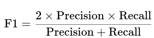
Precision is (True Positives) / (True Positives + False Positives), indicating among the samples predicted as positive, how many truly were positive. Recall is (True Positives) / (True Positives + False Negatives), indicating among the samples that were truly positive, how many did we catch as positive predictions.
When interpreting F1 score values, note that:
It ranges between 0 and 1.
1 indicates the best possible performance (perfect Precision and perfect Recall).
0 means the worst performance (no trade-off achieved between Precision and Recall).
In many real-world scenarios, you may see a moderate F1 score when there is a significant class imbalance or one type of error is more prevalent. It is often a more realistic metric compared to Accuracy when the data is highly skewed, because the F1 score pays attention to both Precision and Recall.
Practical Implementation Example
from sklearn.metrics import f1_score

# Suppose we have the true labels and our model's predictions
y_true = [0, 1, 1, 0, 1, 1, 0]
y_pred = [0, 1, 0, 0, 1, 1, 1]

f1 = f1_score(y_true, y_pred)
print(f"F1 Score: {f1}")
This Python snippet uses scikit-learn to compute the F1 score. Internally, scikit-learn calculates Precision and Recall, then applies the formula for the F1 measure.
Why F-Score Is Useful
The F-score is extremely helpful in cases where we care about both types of errors (false positives and false negatives) and do not want to rely on one-dimensional metrics such as Accuracy, which may be misleading if the classes are imbalanced. By harmonizing Precision and Recall, the F1 score provides a single number to evaluate the model’s quality in identifying positives correctly.
If different weighting is needed (for instance, if missing positives is far more severe than wrongly labeling negatives as positives), you could use the more general F-beta score, which allows you to emphasize Recall more (beta>1) or Precision more (beta<1).
How to Interpret F-Measure Values
Since the F1 score is bounded between 0 and 1:
A value close to 1 implies both high Precision and high Recall, indicating that the classifier rarely misses positives and rarely flags negatives as positives.
A value substantially below 0.5 typically indicates that the model is either missing a large number of positives or predicting many negatives as positives.
Intermediate values should be analyzed together with Precision and Recall to see which dimension is pulling the F1 score down or up.
Possible Pitfalls
If the dataset is extremely imbalanced, even an F1 score might mask certain issues if Precision or Recall is far from the desired range. Always pair the F1 score with separate reporting of Precision, Recall, or a confusion matrix to understand the model’s mistakes in depth.
Follow-up Question: Why might one choose F1 over Accuracy?
Accuracy may be misleading when the data is imbalanced. In a situation where the positive class is very rare, a high Accuracy could be achieved by always predicting the majority class (thus ignoring most positives). However, the F1 score punishes poor Recall or poor Precision, ensuring you cannot simply rely on predicting mostly negatives to get a seemingly high performance metric.
Follow-up Question: What if I need to prioritize Recall over Precision?
When the cost of missing a positive is very high (for example, missing fraudulent transactions), you may want a higher Recall. In that scenario, you can use the more general F-beta measure. By choosing beta>1, you place more emphasis on Recall. A large beta value ensures that the measure rewards your model’s ability to detect positives more than punishing its false positives.
Follow-up Question: How do we handle extremely imbalanced data with the F1 score?
With highly imbalanced data, the F1 score can be low if your model struggles to detect positives (leading to low Recall), or if it has many false positives (leading to low Precision). You can:
Adjust decision thresholds to find the desired Precision-Recall trade-off.
Use sampling techniques (oversampling the minority class or undersampling the majority class).
Consider alternative metrics like the Precision-Recall AUC for further insight.
Follow-up Question: When might the F1 score be misleading?
If your use case requires significantly different weights for Precision and Recall, the F1 score (which balances them equally) could be misleading. For example, in medical testing for a critical disease, you might prefer to detect as many true cases as possible even if you increase false positives. In that case, F1 might not capture the desired emphasis on Recall. Consequently, a metric like the F-beta score (with beta>1) or a cost-sensitive approach might be more suitable.
Below are additional follow-up questions
How does the F1 score handle multi-class classification scenarios, and what are macro-F1, micro-F1, and weighted-F1?
Multi-class classification expands the notion of Precision, Recall, and F1 beyond binary predictions. Instead of calculating these metrics for only one positive class, each class is treated as its own “positive” class in turn, then the results are averaged in different ways.
Macro-F1: You compute the F1 for each class independently and then take the arithmetic mean of those F1 values. This treats all classes equally, regardless of their frequency. Consequently, it might undervalue overall performance if some classes have very few samples.
Micro-F1: You aggregate the total true positives, false positives, and false negatives across all classes, then compute a single F1 score from these sums. This tends to weight performance according to the more frequent classes because it sums up all positives and negatives across classes before calculating Precision and Recall.
Weighted-F1: You compute the F1 for each class, then average them according to the support (the number of instances) of each class. It is often used when one wants to account for class imbalance more directly than macro-F1.
Below is a central formula for the weighted F1 in multi-class settings:

Where:
K is the total number of classes.
n_i is the number of samples belonging to class i.
F1_i is the F1 score for class i.
Potential Pitfalls:
If classes have widely differing sizes, using macro-F1 might overly penalize performance on tiny classes or artificially inflate the average if performance on rare classes happens to be better.
Micro-F1 can obscure poor performance on small classes if large classes dominate.
Weighted-F1 can mask performance issues on small classes, but provides a more “balanced” view of overall performance when class imbalance exists.
Real-World Edge Cases:
If you have hundreds of classes, each with a different number of samples, choosing macro vs. micro vs. weighted averaging can drastically change perceived model quality.
In certain domains (like topic classification where some classes are extremely rare), you may want to carefully validate metrics with domain knowledge rather than purely relying on a single averaged F1 score.
In an environment with real-time streaming data, how would you maintain or update the F1 score metrics?
When a model is continuously receiving new data, F1 metrics should be recalculated (or updated) in an online or incremental fashion. Two general approaches:
Rolling Window: You maintain a window of recent predictions and labels (for example, the last N samples or data from the past X hours). You then recalculate Precision, Recall, and F1 based on only that window. This method captures recent performance but can be sensitive to window size and shifting distributions.
Incremental Counts: You keep running tallies of true positives, false positives, and false negatives. Periodically, you compute updated Precision, Recall, and F1 from these totals. You might also introduce a decay factor to downweight older data if distribution shifts are expected.
Potential Pitfalls:
Distribution shift: If the underlying data distribution changes drastically over time, older performance metrics might no longer be relevant.
Memory constraints: Keeping detailed statistics of each sample in high-throughput systems can be infeasible, requiring efficient data structures to maintain necessary counts.
Delayed labels: In some streaming environments (e.g., fraud detection), labels for predictions come much later, making it hard to maintain real-time metrics.
Real-World Edge Cases:
Sudden spikes in certain data types (a promotional campaign might cause a flood of new positive instances). Your model's performance could appear to degrade or improve abruptly, affecting the F1 calculations if not carefully managed.
Partial data availability (some labels may be missing until further processing or manual verification happens).
How do you interpret a situation where Precision is extremely high but the F1 score remains moderate?
A moderate F1 in the presence of very high Precision typically indicates Recall is relatively low. This means when the model does predict positives, it is often correct (hence the high Precision), but it may be failing to catch many of the actual positives in the dataset, resulting in a lower Recall.
Potential Pitfalls:
You might be happy about a very low false positive rate, but if missing positives is costly (e.g., identifying diseases, fraud transactions), ignoring those missed positives can be damaging.
If the dataset is imbalanced, you might incorrectly assume high Precision is sufficient without realizing large numbers of positives remain undetected.
Real-World Edge Cases:
Healthcare diagnostics: High Precision but moderate F1 might be unacceptable if missing a single positive case of a critical disease has severe consequences.
Cybersecurity: You might want to catch most breaches (high Recall), so a model that is highly precise but has moderate or poor F1 can be risky.
Could you compare the F1 score to the ROC AUC metric, and discuss where each might be misleading?
The ROC AUC measures the area under the Receiver Operating Characteristic curve, which plots the True Positive Rate against the False Positive Rate at various thresholds. F1 focuses on Precision and Recall at a particular threshold.
F1 is threshold-specific, typically reflecting a single operating point of the classifier.
ROC AUC is threshold-independent in principle, summarizing performance across all possible thresholds.
Potential Pitfalls:
When the dataset is highly imbalanced, ROC AUC can be misleadingly high if the negative class is vast. You might have an impressive ROC AUC even if the model barely catches positives.
F1, being threshold-based, might not give insight into how the model would behave if you shift the decision boundary for different business requirements (e.g., if you want fewer false positives in certain scenarios).
Real-World Edge Cases:
In spam detection, a high ROC AUC might appear good, but the actual threshold you choose for classifying an email as spam can drastically affect Precision and Recall. You might inadvertently delete legitimate emails if the threshold is not tuned properly.
In medical applications, you might need to evaluate how the model performs at different points on the ROC curve. F1 alone does not provide a complete picture of all possible trade-offs, but it gives you a specific view of Precision and Recall trade-offs at a chosen threshold.
What strategies exist for choosing a threshold to optimize the F1 score when the model outputs continuous probabilities?
When a model produces continuous scores (e.g., probabilities), you can systematically scan possible thresholds between 0 and 1, compute the F1 score for each threshold, and then pick the threshold that maximizes F1. Some approaches:
Grid Search: Try thresholds at increments (e.g., 0.0, 0.01, 0.02, …, 1.0).
Ternary or Binary Search: If the function is unimodal in that range, you can use search algorithms to find the maximum more efficiently.
Genetic or Bayesian Optimization: For more complex or large-scale settings.
Potential Pitfalls:
Overfitting to the threshold on the training or validation data. Once you deploy to a different distribution, that threshold might no longer be optimal.
Frequent re-tuning might be required if data shifts over time.
The cost of false positives vs. false negatives might differ in the real world, so maximizing F1 might not be aligned with business objectives if the cost matrix is asymmetric.
Real-World Edge Cases:
If the distribution of predicted probabilities is heavily skewed (model outputs probabilities near 0 or near 1), the threshold search might be sensitive around narrow ranges.
If data is non-stationary, you might find yourself frequently adjusting thresholds to maintain optimal performance.
How does F1 fare if the “positives” themselves are heterogeneous in importance?
Sometimes even within the positive class, different subtypes might have drastically different significance. If you treat them all equally under a single positive class, you might mask poor performance in critical subsets.
Potential Pitfalls:
You might end up with a reasonable overall F1 while failing severely on a more critical subset of the positive class.
Standard F1 treats all positives equally, ignoring real-world cost variations across different “positive” sub-types.
Real-World Edge Cases:
In fraud detection, some fraud cases (involving large amounts) are more impactful than smaller fraud. A single F1 measure lumps these together, potentially obscuring the model’s performance on large-sum fraud.
In medical diagnosis, certain disease subtypes within a single broad category might be more urgent than others. A single F1 could hide a poor detection rate for a life-threatening subtype.
How can we ensure non-technical stakeholders correctly understand the implications of an F1 score?
Stakeholders often are more familiar with simpler metrics (e.g., Accuracy, or the concept of false alarms vs. missed detections). Presenting F1 alone might lead to misunderstanding.
Potential Pitfalls:
Overemphasizing a single value like F1 might fail to communicate the model’s different error trade-offs clearly.
Non-technical audiences might assume an F1 of 0.8 means the model is “80% accurate,” leading to confusion if they mistake it for the conventional notion of Accuracy.
Real-World Edge Cases:
In finance or government compliance audits, stakeholders want to know if certain critical mistakes are being made. A single F1 score does not directly reveal which types of errors are most frequent.
In marketing, the business might care more about missing a potential high-value customer (false negative) rather than occasionally targeting an uninterested individual (false positive). If F1 is good but the false negative rate is still high in that segment, it can cause strategic mistakes.