
ML Interview Q Series: Could you explain the nature of the bias-variance tradeoff in machine learning and suggest approaches to address excessive bias?


📚 Browse the full ML Interview series here.
Comprehensive Explanation
The concept of bias-variance tradeoff underlies model complexity and its generalization performance. Bias refers to the model’s tendency to systematically deviate from the actual target values due to oversimplified assumptions. Variance indicates how sensitively the model’s predictions fluctuate with respect to changes in the training set. When a model has high bias, it typically underfits, performing poorly because it does not capture the underlying data patterns sufficiently. When a model has high variance, it overfits, modeling noise in the training data and failing to generalize well to unseen data.
A widely recognized perspective on this relationship comes from the bias-variance decomposition of expected error:
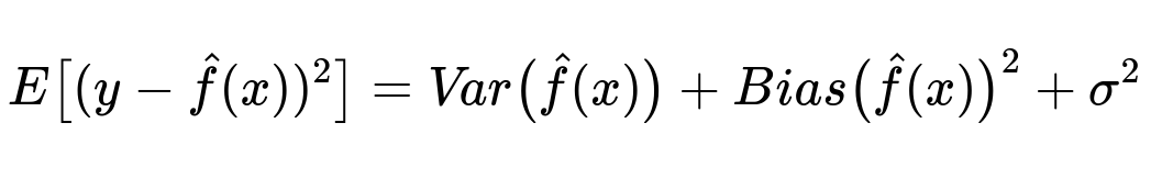
Here, y is the true label, x represents the input features, and \hat{f}(x) is the model’s prediction. Var(\hat{f}(x)) indicates the variance component (how much the model’s predictions vary for different training sets), Bias(\hat{f}(x))^2 is the squared bias (how far the model’s average predictions are from the true values), and \sigma^2 is the irreducible error (noise inherent in the data that cannot be explained by any model).
High bias means that Bias(\hat{f}(x))^2 is large. The model’s assumptions are too restrictive, leading to underfitting. Possible remedies for high bias include:
Increasing model complexity. One might move from a simple linear model to a more complex classifier or regressor (e.g., adding polynomial features, switching to neural networks, or using ensemble methods).
Reducing regularization strength. If strong regularization (L2, L1, dropout in neural networks) is preventing the model from learning essential patterns, relaxing that regularization can help the model capture more nuanced relationships.
Introducing relevant features. More informative or engineered features can help a simpler model reduce bias, as it is given more helpful predictors to model the data accurately.
Decreasing data preprocessing constraints. If the data preprocessing pipeline is too restrictive (e.g., overly aggressive dimensionality reduction), it might be contributing to the model’s inability to learn.
When addressing the bias-variance tradeoff, it is important to avoid simply driving down bias at the expense of ballooning variance. Good generalization arises from balancing complexity (to reduce bias) with appropriate regularization (to control variance).
What are some typical symptoms of a high-bias model?
A high-bias model often manifests poor performance both on the training set and the test set, indicating underfitting. The model’s predictions fail to capture the complexity in the training data itself. A typical sign is that training metrics and validation/test metrics are both unsatisfactory, and further training doesn’t reduce the training error significantly.
In practice, how can we detect that a model is suffering from high bias rather than high variance?
One straightforward approach involves comparing training and validation performance. If training accuracy (or training performance metrics) is too low and close to the validation accuracy, it usually signals high bias. In contrast, if training performance is very high but validation performance lags significantly, that is a hallmark of high variance or overfitting.
Additionally, plotting learning curves is helpful. If the training and validation curves converge to a relatively high error level, it suggests bias. If they diverge significantly, it suggests variance.
Why does increasing model complexity help reduce bias?
When a model is too simple (e.g., a linear model without sufficient interaction or higher-order terms, or a shallow decision tree), it fails to capture more complex patterns. By increasing complexity, for instance by adding more parameters, increasing the depth of a neural network, or using random forests instead of a single decision tree, the model gains flexibility to approximate the underlying function more precisely. This additional capacity typically reduces the systematic error (bias), though it might increase variance if not carefully managed.
What if the model still underfits even after increasing complexity?
In some cases, insufficient training data or poor data quality may limit the capacity of a model to reduce bias. One should ensure the dataset is sufficient in size and contains relevant features. In deep learning, for example, a model might be large enough but still underfit if the learning rate is not tuned, or if certain architecture choices (like improper activation functions) constrain its effective capacity. Conducting thorough hyperparameter tuning, performing proper data preprocessing, and ensuring that the architecture is well-aligned with the problem domain are essential steps.
How do we mitigate the risk of increasing variance while reducing bias?
One should apply the right level of regularization and adopt good generalization strategies such as dropout (in neural networks), early stopping, ensemble methods, or cross-validation. These help ensure that as complexity increases, the model does not overfit excessively. Techniques like cross-validation can provide a reliable estimate of how changes in model complexity affect generalization performance.
How does feature engineering interplay with high bias?
Introducing new, more expressive features can significantly improve a model’s ability to capture underlying patterns. For instance, if a linear model is biased because it lacks interaction terms among features, manually crafting those interactions or using polynomial features can reduce bias. However, one must be cautious not to add a large number of arbitrary features that might lead to an increased risk of overfitting.
Could ensembles of weak learners help with high bias?
A well-chosen ensemble method, such as boosting (e.g., Gradient Boosting Machines or AdaBoost), can effectively reduce bias by combining many weak learners in a sequential manner. Boosting especially focuses on correcting errors made by previous learners, often alleviating underfitting in the process. At the same time, one has to keep an eye on the variance that may arise as the model grows more complex. Random Forest, another ensemble technique, often provides a good balance between bias and variance by averaging predictions across multiple diverse trees.
How do we evaluate if our actions to reduce high bias are successful?
Tracking training metrics along with validation/test metrics is key. By employing cross-validation, one can measure how changes (e.g., adding more features, reducing regularization, changing model architecture) impact performance consistently across folds. If training error decreases significantly but validation error remains roughly the same, it could indicate that variance is now an issue. Conversely, if both training and validation errors reduce, it suggests that the adjustments helped mitigate bias.
What else can be done if high bias persists?
Another approach is to try fundamentally different learning algorithms. For instance, if one keeps using simple linear or tree-based models and still observes high bias, switching to methods like neural networks (for complex, high-dimensional data) or kernel methods like SVM (with an appropriate kernel) might provide a more powerful function space. Additionally, gathering more data, especially if the dataset is not representative enough, can often improve the learning process by allowing more complex models to train effectively without overfitting too quickly.
Below are additional follow-up questions
Could adding more data ever unintentionally increase bias, and under what conditions might that happen?
When we add more data, the typical expectation is that the model gains more diverse examples, thereby reducing variance and potentially addressing underfitting issues. However, if the additional data is not representative of new patterns and instead reinforces the same underlying distribution or biases already present, the model might still remain oversimplified. In scenarios where the extra data comes from the same biased source, the model might effectively “learn” similar simplified assumptions more strongly. If the data continues to emphasize certain features or patterns and the model’s architecture or hyperparameters remain insufficient to capture relevant complexity, the model may not see any reduction in bias. This often occurs in real-world settings where gathering new data from a broader domain is costly, leading teams to append more of the same type of data. The key is to ensure that any newly acquired data extends the variety in meaningful ways (e.g., new classes, different conditions, varied contexts) rather than merely inflating the dataset size.
How does domain expertise intersect with reducing bias, and when might ignoring domain knowledge lead to high bias?
Domain expertise helps identify which patterns or features truly matter in a given application. If a model is constructed purely by generic data-driven methods without leveraging relevant domain insights, it might fail to capture important relationships, resulting in high bias. For instance, in medical image classification, certain morphological details might be crucial, yet a purely data-driven approach might disregard them if they appear in too few samples. By incorporating domain knowledge—like known biomarkers, specific anomaly regions, or established transformation methods—the model can be given a richer feature space or more nuanced pre-processing. Conversely, relying exclusively on domain assumptions can also become detrimental if such assumptions are too narrow or outdated, thereby reinforcing the model’s bias. Hence, the interplay between domain expertise and data-driven exploration is critical to properly reduce bias without inadvertently missing emerging or subtle patterns.
Could a non-convex learning objective contribute to persistent high bias, and how can we address it?
In many deep learning frameworks or other complex models (e.g., certain forms of latent factor models), the training objective is non-convex. One might initially assume that non-convexity primarily impacts variance (due to local minima or saddle points). However, if the optimization process continually gets stuck in local minima, the model’s effective capacity might be underutilized, yielding systematic underfitting (high bias). For example, in deep neural networks, poor weight initialization or suboptimal learning rate scheduling can result in subpar minima that do not capture intricate patterns. To address this:
Use advanced optimizers like Adam or RMSProp, which adapt the learning rate for each parameter.
Adopt techniques such as learning rate warm-up, restarts, or cyclical learning rates to escape suboptimal minima.
Utilize better weight initialization methods or carefully tuned heuristics (e.g., Xavier/Glorot, He initialization for ReLU layers).
Consider re-initializing and retraining multiple times to see if a better solution (with lower bias) can be achieved.
How does high dimensionality impact bias, and can underfitting still occur even with more features than samples?
In principle, having a large feature space provides a model with the potential to capture more complex relationships, which often reduces bias. However, if we naively add features that lack relevance to the task or are mostly noise, the model may not genuinely expand its capacity to represent meaningful patterns. Moreover, in extremely high-dimensional spaces with limited data, the effective sample complexity can become so challenging that certain model assumptions or regularizations forcibly simplify the model. For instance, if strong regularization is used to prevent overfitting in a high-dimensional setting, the net effect can push the model toward oversimplification and produce high bias. Another edge case arises with something like PCA-based dimensionality reduction if the explained variance threshold is too restrictive. In that situation, you might discard critical patterns that exist in lower-variance components. Even though the data is high-dimensional, you are effectively pushing the model into a low-dimensional approximation that might be too simple, thereby causing high bias.
Could an extremely noisy dataset make it seem like the model has high bias, and how to differentiate true underfitting from irreducible noise?
Excessive noise in the labels or features can lead to high training and validation error alike, which superficially resembles a high-bias scenario. But in reality, some fraction of that error is irreducible noise that no model can learn. Distinguishing the two requires carefully inspecting the data generation process, verifying whether the labels are consistent and the features are measured accurately. Techniques that help:
Collect multiple labels for the same instances and see if there’s an inherent disagreement or labeling errors.
Conduct data-cleaning steps to remove or correct obviously corrupted entries.
Use domain knowledge or external references to gauge the inherent variability in the phenomenon being studied. If the irreducible noise portion is large, you can keep increasing model complexity but the improvement might be marginal. Understanding this boundary helps avoid over-investing in complexity when the data simply does not support lower error due to noise.
In what circumstances might an ensemble model still exhibit high bias, and what would be a strategy to fix it?
Ensemble methods like bagging or boosting are often heralded for reducing variance more than bias, but they can still produce high bias if each base learner is fundamentally too restricted. For example, using many shallow decision trees in a bagging ensemble might not reduce bias much if none of those trees individually has enough depth to represent complex relationships. Similarly, if we use an ensemble of linear models but the actual data-generating process is non-linear with intricate interactions, the ensemble could remain biased. A strategy to fix this involves either:
Increasing the capacity of individual weak learners (e.g., deeper trees, polynomial basis expansions).
Switching the ensemble type: from bagging to boosting, which can more aggressively reduce residual errors.
Enriching the feature space with domain-informed transformations or interactions so that even a simpler base learner can capture more patterns.
When focusing on interpretability, might we perpetuate high bias, and what tradeoffs do we face?
Interpretable models such as shallow decision trees or linear regressions with minimal interaction terms are easier to communicate and justify in regulated industries. However, their simplicity often puts them at a higher risk of underfitting. This can be problematic if the underlying relationships are significantly non-linear or complex. The tradeoff is that while deeper or more complex models reduce bias by capturing richer patterns, their interpretability can suffer. A potential middle ground might involve methods like:
Model distillation, where you train a complex model and then approximate its predictions with a simpler one to glean interpretability insights.
Local interpretable model-agnostic explanations (LIME) or SHAP methods that offer instance-level interpretability without forcing the global model to remain overly simple. Balancing interpretability with adequate model complexity is crucial to avoid a scenario where the bias is so high that the model becomes nearly useless for real predictive tasks.
How might we monitor a deployed model over time to detect emerging high bias, and what are the real-world pitfalls?
Once a model is deployed, data distributions may drift or shift. If the new incoming data patterns differ from those in the training set, the model could start underfitting relative to the new distribution. Suddenly, the model’s previously adequate complexity might appear too low when confronted with unseen trends or relationships. Monitoring strategies include:
Continuous evaluation on fresh data and comparing performance metrics to historical baselines.
Implementing “canary” or “shadow” models—alternative models that run in parallel to assess if there’s a consistent performance discrepancy.
Checking feature statistics (such as mean, variance, correlation) over time to see if data drift is occurring. Pitfalls arise if the organization does not maintain a robust feedback loop or neglects to label new data. In those cases, detection of bias creep or drift might be delayed, causing systematic degradation of predictions.
What is the distinction between irreducible error and model bias, and how do we avoid misidentifying one as the other?
Irreducible error stems from inherent uncertainty or noise in the data generation process. Model bias, on the other hand, is error attributable to oversimplified assumptions or insufficient model complexity. A real-world pitfall is repeatedly adding complexity (e.g., layering more network depth or assembling multiple learners) in an attempt to reduce error when that error is mostly driven by random noise or measurement inconsistencies. This can waste resources and, worse yet, can increase variance unnecessarily. The best way to mitigate this confusion is to:
Perform thorough data exploration to understand the baseline “noise floor.”
Use domain knowledge to confirm whether certain phenomena are inherently unpredictable.
Compare different model complexities and watch if the training error decreases but the validation error plateaus. If the error stalls, it may indicate saturation due to irreducible noise rather than model bias.
Why might adding more features not always solve the high bias problem, and could it create other issues?
Although adding features can increase a model’s representational power, blindly adding them may fail to address the crux of underfitting if those new features are not relevant or do not capture more meaningful information about the target. Moreover, if the new features are correlated or noisy, the model might struggle with spurious relationships, leading to confusion between relevant signals and noise. This can complicate model training and potentially induce more variance. For example, in a recommendation system, adding thousands of generic user features that barely correlate with preferences might not reduce bias at all. Instead, the model’s complexity would grow, requiring stronger regularization or more training data, possibly pushing you back toward higher bias inadvertently. The solution is carefully targeted feature engineering, guided by domain knowledge, statistical analysis, and iterative experimentation to ensure that any newly introduced features genuinely enrich the model’s view of the predictive task.