
ML Interview Q Series: DAU drops 1% weekly—how to confirm significance vs. randomness and approach the analysis?
📚 Browse the full ML Interview series here.
Comprehensive Explanation
One of the most direct ways to determine if a gradual weekly decline in DAU (Daily Active Users) is non-random is to perform statistical hypothesis tests that can detect trends over time. In addition, we can apply exploratory data analysis to see if the trend is consistent and if there are any seasonality patterns or anomalies. Below is a structured approach:
Data Collection and Exploration
Obtain sufficient historical DAU data to ensure statistical robustness and to account for any seasonality or external factors (e.g., weekends, holidays, or app version releases). Visualize the data over time to see the trend, check for outliers, and identify cyclical or seasonal patterns that might mask or exaggerate a 1% weekly drop.
Formulating a Hypothesis
Typically, you can set up a null hypothesis H0 stating that there is no real decline in the DAU trend and that any observed decrease is purely due to random variation. The alternative hypothesis H1 is that there is a genuine decreasing trend in DAU over time.
Applying a Statistical Test for Trend
A common way to determine if the slope of a time series is significantly different from zero is to fit a simple linear regression model where time (in weeks) is the predictor variable and DAU is the response variable. If the slope of the fitted line is significantly negative, it suggests a true downward trend. The general simple linear regression formula can be expressed by:

Here:
y represents the DAU.
x represents time (for instance, week number).
beta_0 is the intercept term.
beta_1 is the slope indicating how much DAU changes week by week.
epsilon is the error term, assumed to be normally distributed with mean 0.
Once this model is fit, you compute the t-statistic for beta_1 to check if it differs significantly from 0. The test statistic is:
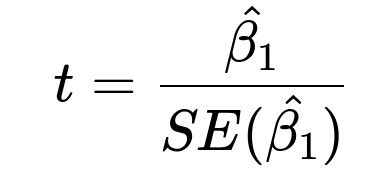
Here:
hat{beta_1} is the estimated slope from the regression.
SE(hat{beta_1}) is the standard error of that slope estimate, derived from the variability in the data.
If the p-value associated with this t-statistic is below a chosen significance level (often 0.05), you reject the null hypothesis and conclude there is a statistically significant downward trend.
Checking Stationarity and Autocorrelation
Many time series have autocorrelation, meaning that observations close in time are correlated. Standard regression assumptions (i.i.d. errors, no autocorrelation) might be violated. If strong autocorrelations exist, a standard OLS approach can overestimate or underestimate the significance of the slope. In that case, methods like ARIMA, ARIMAX, or generalized least squares (GLS) regression might be more appropriate.
Considering a Week-by-Week Difference Test
Another approach is to compare consecutive weeks’ DAUs to see if the difference is consistently negative over multiple weeks. If the data for each week are independent samples of user activity and the distribution is roughly normal for large user bases, you can do pairwise t-tests comparing average DAU from one week to the next. Over multiple weeks, if you consistently observe a negative difference, you can perform:
A sign test (non-parametric) to see if the sign of the weekly change is predominantly negative.
A one-sample t-test on the weekly difference (week_i – week_(i-1)) to check if its mean is significantly below zero.
Confidence Intervals
To enhance your confidence in the trend, construct confidence intervals around the slope. If the interval does not include zero (or includes only small positive slopes that are inconsistent with the observed data), this gives additional evidence that the decline is real.
Controlling for Covariates
Many factors can affect DAUs, such as marketing campaigns, feature releases, or seasonal usage patterns. If applicable, include relevant control variables in the model. That would transform the simple regression into a multiple regression, where each additional factor is accounted for to isolate the effect of “time.”
Practical Considerations
In real-world systems, even a small negative slope can have compounding effects. After confirming a downward trend, it is vital to investigate user feedback, usage logs, or funnel metrics to identify whether new bugs, changes in user experience, or external factors are driving the decline.
Example Analysis in Python
import pandas as pd
import statsmodels.api as sm
import numpy as np
import matplotlib.pyplot as plt

# Suppose df has columns: ['week', 'dau']
# We'll do a simple linear regression of DAU over weeks.
df = df.sort_values(by='week')
X = df['week']
y = df['dau']

# Add constant to predictor
X = sm.add_constant(X)

model = sm.OLS(y, X).fit()
print(model.summary())

# Check the slope (model.params['week']) and its p-value from model.
# If p-value < 0.05, we say there is a statistically significant trend.
In production scenarios, you might opt for time series methods or incorporate additional covariates. However, the code snippet above demonstrates a simple OLS approach to see if there is a significant linear decline in DAU.
Potential Follow-Up Questions
How do you handle the possibility of seasonality affecting DAU?
Seasonality can cause periodic fluctuations, such as weekends or holidays where user activity might deviate from normal patterns. If seasonality is present, consider:
Including seasonal dummy variables. For instance, if you suspect differences by day of the week or month of the year.
Using time series models (e.g., SARIMA) that explicitly model seasonality.
Decomposing the time series to extract the seasonal component and then analyzing the trend in the seasonally adjusted data.
What if the data shows autocorrelation in the residuals?
If residuals are autocorrelated, standard linear regression might not yield correct standard errors, leading to inaccurate p-values. You can:
Use ARIMA or SARIMA if the data is well-described by these processes.
Use generalized least squares regression with a correlation structure suited to the data.
Apply the Durbin-Watson test or Ljung-Box test to diagnose autocorrelation and choose the appropriate remedy.
Could a small sample size affect the test's power?
Yes, a small sample size can lead to insufficient power to detect a 1% decrease, especially if daily or weekly usage has high variance. Solutions include:
Aggregating more historical data (if available).
Combining multiple metrics or running the test for a longer period, if it is business-acceptable.
Checking effect size measures (e.g., Cohen’s d) to understand the practical significance even if the test lacks power.
How do you structure your final recommendations to stakeholders?
You would present:
The statistical evidence for a downward trend (including confidence intervals and p-values).
Possible external or internal factors discovered during analysis that might explain the decline.
Actionable suggestions, such as user surveys, feature rollbacks, or new experiments to diagnose user behavior changes more precisely.
A plan to continually monitor DAU with an automated alert system that triggers further investigation if DAUs deviate below a threshold.
What if there is missing data for certain weeks?
Missing data can distort time series analysis. You could:
Impute missing values using linear interpolation, forward fill, or more advanced methods like Kalman filters.
Omit the missing weeks if the data is sporadic, though this can introduce bias if a large portion is missing.
Use models that can handle irregular time steps, or robust time series methods that incorporate missingness in a principled way.
By thoroughly verifying statistical significance, adjusting for potential confounders, and exploring root causes, you can be confident in your conclusion about whether a 1% weekly DAU drop is real and requires immediate attention.
Below are additional follow-up questions
What if user segments differ drastically in their usage patterns?
Different segments of users (e.g., new vs. returning, geolocation-based, platform-based) may exhibit unique behaviors, which can mask or exaggerate an overall 1% decline. For instance, if you have a fast-growing segment that still shows healthy engagement while another segment is silently churning, the average DAU might only appear to be dropping slightly each week. To address this:
Segmentation Analysis: Split DAUs by relevant attributes (e.g., region, device, subscription level) to see if the decline is concentrated in specific groups.
Customized Statistical Tests: Within each segment, apply the same hypothesis testing for trends. Some segments might show stability, while others show steeper decline.
Cross-Segment Interactions: If marketing or product updates mainly affect certain user groups, factor those into your regression models by adding interaction terms with user segment indicators.
Potential Pitfalls:
Over-segmentation can reduce sample size in each subgroup, leading to lower statistical power.
Combining segments with widely different behaviors might dilute meaningful signals.
How do you control for marketing campaigns or inorganic spikes in user acquisition?
Marketing efforts, promotions, or paid user acquisition can artificially inflate DAU in the short term, followed by a correction that might look like a decline when the campaign ends. This effect can obscure real patterns. To mitigate this:
Mark Key Campaign Dates: Record when each marketing campaign started, ended, and its scope or magnitude.
Include Indicators in the Model: In a regression context, add binary variables capturing whether a campaign was active during a particular week. This helps differentiate trend from campaign-related boosts.
Look at Unadjusted vs. Adjusted Trends: Compare raw DAU trends with marketing-adjusted time series to see if the decline remains significant after removing these effects.
Potential Pitfalls:
Campaign measurement error if you do not accurately track spend or impressions.
Lag effects where the impact of a campaign continues even after it ends.
How do you deal with extreme outliers or highly skewed data?
Even a small set of days with unusually high or low DAU could distort your weekly averages or your regression assumptions. For instance, a single day of a major outage or a viral event can shift the mean enough to misrepresent the underlying trend. Strategies include:
Identify Outliers: Use statistical methods (e.g., IQR-based filtering, z-scores) or domain knowledge to detect days with abnormally high or low values.
Winsorizing or Capping: Instead of removing outliers, cap extreme values to a certain percentile to reduce undue influence.
Robust Regression Techniques: Methods like Huber regression or RANSAC can handle outliers better than standard OLS.
Potential Pitfalls:
Removing true anomalies might mask real issues (like an outage).
Over-filtering can distort genuine signals about user engagement spikes.
How do you handle scenarios where the product experience or feature set changes significantly?
Major changes in product design or feature rollouts can alter user behavior in ways that don’t align with a simple linear time-based decline. For example, introducing a new onboarding flow might initially lower DAU if some users drop off, but could lead to higher long-term retention. You can:
Segment by Release Cohorts: Track DAUs for users who joined before vs. after a major product change.
Model as a Step Change: In a time series framework, treat the product change date as an intervention point in an Intervention Analysis.
Multi-Phase Regression: Split the timeline into pre-change and post-change intervals, fitting separate models to gauge the difference in slopes.
Potential Pitfalls:
Overlooking changes that roll out gradually (feature flags or staggered releases).
Correlating a drop with a product change that is actually coincidentally timed with an external factor.
How do you design an experiment to recover from or confirm a cause of the decline?
If a hypothesis is that a particular user experience issue or product deficiency is driving the decline, an experiment can test potential fixes:
Controlled Rollout: Release the solution (e.g., a revamped feature) to a random subset of users. Compare their DAU trend to a control group that doesn’t receive the fix.
Define Clear Metrics: Besides overall DAU, track daily sessions, session length, churn rate, or conversion funnels for deeper insights into user behavior.
Avoiding Confounds: Ensure other parallel changes do not simultaneously roll out to the same experimental group unless that is part of the design.
Potential Pitfalls:
Insufficient sample size in the test group, leading to inconclusive results.
External events overshadowing the effect of the fix (e.g., holiday season, competitor promotions).
How do you interpret the situation if the time series is non-linear?
A 1% week-on-week decline may not be constant but might accelerate or decelerate, leading to curved patterns. Standard linear regression could miss these nuances:
Polynomial or Piecewise Linear Models: Expand your model to allow quadratic or even higher-order terms, or break the timeline into segments with different slopes.
Non-Parametric Approaches: Use smoothing techniques (e.g., LOESS, spline regressions) to uncover more complex patterns without specifying a functional form.
Potential Pitfalls:
Overfitting with too many polynomial terms.
Misinterpreting cyclical behavior as a sign of a deeper trend.
How do you proceed if the data distribution or error variances don’t meet standard OLS assumptions?
Time series can show heteroskedasticity (unequal variances over time), or the DAU data might not be normally distributed, especially if user counts are extremely large or heavily skewed. Possible solutions:
Transformations: Take the log of DAU if the data spans multiple orders of magnitude. This can stabilize variance.
Robust Standard Errors: Use heteroskedasticity-robust or Newey-West standard errors to handle potential correlations and changing variances.
Generalized Linear Models: If DAU has a count-like distribution, a Poisson or negative binomial regression might be more suitable.
Potential Pitfalls:
Log transformation complicates interpretation (differences become multiplicative rather than additive).
Over-dispersion in count models leading to incorrect p-values.
How could data privacy or sampling policies affect your analysis?
Privacy regulations or system constraints may require storing only aggregated data or randomly sampling user behavior, which can hide or reduce visibility into subtle trends:
Aggregated vs. User-Level Data: Aggregation smooths out random day-to-day fluctuations, potentially obscuring localized drops in a particular segment.
Sampling Bias: If certain user types opt out of tracking, your sample may underrepresent or overrepresent specific demographics, skewing your trend analysis.
Potential Pitfalls:
Inability to drill down into specific user cohorts if only anonymized totals are available.
Non-random sampling leading to biased estimates of the trend.
What is the role of retention analysis or survival analysis in diagnosing this decline?
Weekly DAU drops might be caused by users leaving (churn) at faster rates than new users join, rather than an overall reduction in daily sessions from active users. Incorporating retention metrics could clarify this:
Cohort Retention Curves: Track the percentage of users from each signup cohort who return daily or weekly. An accelerating drop in retention is a leading indicator of the DAU decline.
Survival Analysis: Model the time-to-churn distribution. If the hazard function (the instantaneous rate of churn) has recently increased, that strongly suggests the downward DAU trend will continue.
Potential Pitfalls:
Ignoring partial churn behavior, e.g., users who only reduce usage but don’t fully depart.
Overlooking new user acquisition offsets that partially mask churn.
How could real-time analytics or streaming data techniques help identify the decline sooner?
Relying on weekly aggregates might delay detection of significant drops until after multiple days. Real-time pipelines can surface abrupt changes:
Streaming Aggregations: Continuously monitor daily or even hourly active users. If the drop accelerates, alerts can fire before a full week’s data arrives.
Online Learning or Anomaly Detection: Use models that update with each new data point to detect sudden downward shifts in near real-time.
Potential Pitfalls:
Noise in short time intervals can lead to false alarms.
Data latency or incomplete ingestion pipelines might produce misleading partial data.