
ML Interview Q Series: Decision Tree Splitting: Using Entropy and Gini Impurity to Maximize Information Gain.

📚 Browse the full ML Interview series here.
Decision Tree Splitting Criteria: How does a decision tree decide on which feature and value to split at a node? *Explain what entropy and Gini impurity are, and how information gain is computed to evaluate the quality of a split. If possible, formulate the information gain calculation for a simple split.*
Heading and sub-heading without numbered points.
Understanding Splitting Criteria
A decision tree selects the best feature (and the corresponding split value for that feature) that maximizes a certain measure of "purity gain" (or reduction in impurity) when forming child nodes from a parent node. Two major impurity metrics used for classification tasks are entropy and Gini impurity. The decision tree algorithm examines all possible splits (i.e., all features and, if continuous, all possible threshold values) and picks the one that leads to the best increase in purity among the resulting subsets.
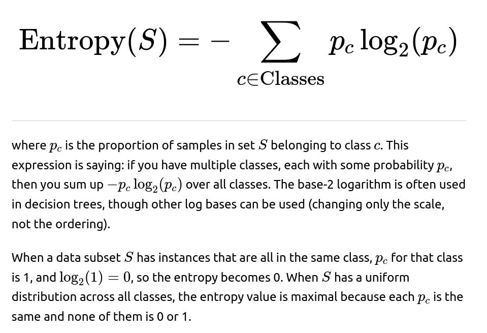
Entropy
Entropy is a concept from information theory. It measures the impurity or disorder in a dataset of class labels. If a node is "pure" (i.e., all samples belong to one class), then the entropy is 0. At the other extreme, when classes are equally distributed, the entropy is larger.
Gini Impurity
Gini impurity is another measure of how often a randomly chosen element from the set S would be incorrectly labeled if we label it randomly according to the class distribution in S. A lower Gini value means a higher purity of the node.

In words:

With Gini impurity, we do something similar:
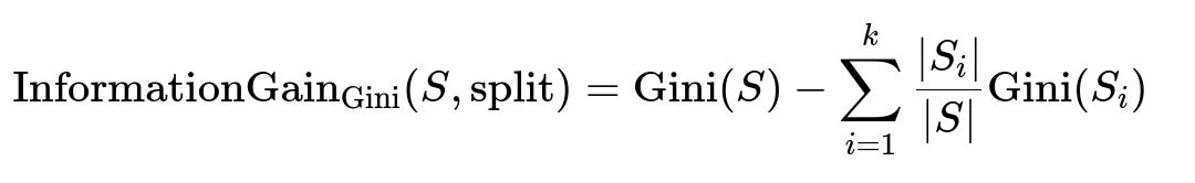
The core idea is the same: pick the split that yields the largest decrease in impurity.
Example of a Simple Split
Imagine a binary classification problem with 10 samples at a node, of which 6 belong to class A and 4 belong to class B. The entropy at this node is:

The weighted average of these two entropies is:
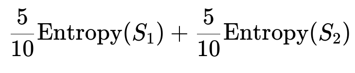
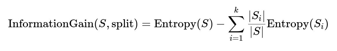
Subtract that from the original entropy of S to get the information gain.
Decision trees will explore the space of possible splits and choose the one that gives the highest information gain (or equivalently, the largest impurity reduction).
Could you elaborate on how to handle continuous features in decision tree splitting?
In real-world datasets, features are often continuous (e.g., numeric features). The typical strategy is to iterate over distinct sorted values of that feature and pick a threshold that partitions the data into two subsets (values less than or equal to the threshold vs. values greater than the threshold). For each potential threshold, the algorithm computes the resulting impurity reduction and retains the threshold that yields the best gain. The search for the threshold is usually performed by sorting the feature values, then considering midpoints between consecutive distinct values as potential split points.
An important note is that a pure brute-force approach could be very expensive if you had to check every possible numeric value. Sorting plus checking midpoints is more efficient (often O(nlogn) for sorting and O(n) for evaluating all candidate thresholds), but still might be expensive in large datasets. In practice, decision tree implementations optimize these steps carefully or apply approximate strategies (especially in gradient-boosting frameworks).
Could you explain the difference between Gini Impurity and Entropy in practice, and which criterion is used more often?
While both Gini and Entropy measure node impurity, there are some practical differences:
Gini is computationally slightly simpler because it lacks the logarithm in the summation. It generally behaves similarly to entropy in terms of choosing splits, especially for many standard classification tasks. In scikit-learn, for instance, the default splitting criterion for the CART decision tree algorithm is Gini. Some references suggest that Gini might have a slight bias toward splits that isolate the most frequent class, whereas entropy might be more sensitive to small class probabilities. In practice, they usually produce very similar trees, and no criterion is strictly superior across all datasets.
In many libraries, Gini is the default due to its computational simplicity and historically consistent performance. Entropy can be used when you prefer a more information-theoretic measure, or to be consistent with certain theoretical references in information theory.
How do we handle overfitting in decision trees, and why are ensemble methods like random forest or gradient boosted trees effective solutions?
Decision trees, if grown fully (allowing each leaf to have very few samples), can overfit by creating highly specific rules that do not generalize beyond the training data. There are various ways to manage this:
Pruning: Post-pruning or pre-pruning can remove or prevent the creation of leaves that don’t bring real predictive power. Pre-pruning stops the tree growth if some metric (like information gain) doesn’t reach a threshold, or if the node size is below a threshold. Post-pruning involves growing a large tree and then pruning back subtrees based on certain metrics like cross-validation error or a complexity penalty.
Limiting Depth or Leaf Samples: Setting a maximum depth or requiring each leaf to have a minimum number of training samples keeps the model from creating overly specific rules.
Minimum Information Gain Decrease: Some implementations require that a split must yield a gain in impurity reduction above a certain threshold. If the threshold is not reached, the node is not split further.
Ensemble Methods: Random forests and gradient boosting ensembles create multiple (or a sequence of) trees. They help reduce variance and avoid overfitting:
Random Forests build multiple independent trees, each from a bootstrap sample of the data and/or a random subset of features. The final prediction is typically the majority vote (or average) of all trees. This averaging reduces the variance of the final model.
Gradient Boosted Trees build a sequence of smaller trees, each focusing on errors of the previous model. By combining many weak learners into an additive sequence, the final strong learner generalizes better than a single large decision tree.
Could you talk about the computational complexity of building a decision tree?
The computational complexity of building a standard decision tree from scratch can be relatively high if done naively. For a dataset with N samples and D features:
At each node, the algorithm searches for the best split among all features and among all possible threshold values. If a feature is continuous, you sort the values or do a partial approach to identify candidate thresholds. Sorting a feature of length N can cost O(NlogN), and doing it for D features yields O(D×NlogN) for evaluating splits at a single node if you do it from scratch.
However, modern implementations often reuse partial computations from parent nodes, or rely on data structures to quickly find the best threshold.
When the tree grows deeper, each level might involve subsets of the data. The total cost can be approximated but is often stated as O(D×NlogN) for building a full tree, depending on the depth and distribution of the data. The best actual complexity can vary if you prune the tree early or use advanced data structures.
Could you talk about the practical differences among different splitting criteria, including Gini, Entropy, or others like classification error?

Gini and Entropy, in contrast, respond more smoothly to changes in node distributions. They more heavily penalize nodes that are "impure," which leads to better decisions about how to split. Because classification error is not as nuanced, it tends to produce less optimal splits, although it remains popular for describing final accuracy at a leaf node.
Could you show some sample code in Python for building a simple decision tree from scratch focusing on the splitting criterion?
Below is a simplified Python example illustrating how you might compute information gain and pick a best split for a single node. This is not a full production-ready tree, but it helps demonstrate the logic of how you might evaluate splits based on impurity:
import numpy as np

def entropy(y):
    # y is a list or array of class labels at the node
    # Convert to np array if needed
    labels, counts = np.unique(y, return_counts=True)
    probabilities = counts / counts.sum()
    ent = 0.0
    for p in probabilities:
        ent -= p * np.log2(p)
    return ent

def info_gain_entropy(X, y, feature_index, threshold):
    # Split into left and right subsets
    left_indices = X[:, feature_index] <= threshold
    right_indices = X[:, feature_index] > threshold

    y_left = y[left_indices]
    y_right = y[right_indices]

    # Calculate overall entropy
    ent_parent = entropy(y)

    # Weighted average of child entropies
    n_left = len(y_left)
    n_right = len(y_right)
    n = len(y)

    ent_left = entropy(y_left)
    ent_right = entropy(y_right)

    weighted_sum = (n_left / n) * ent_left + (n_right / n) * ent_right

    # Information gain
    gain = ent_parent - weighted_sum
    return gain

def best_split(X, y):
    # For demonstration, we'll pick the best feature and threshold
    # from all possible (feature, threshold) pairs in a brute-force manner
    best_gain = -1
    best_feature = None
    best_thresh = None

    n_samples, n_features = X.shape

    for feature_index in range(n_features):
        # Potential thresholds are unique values in this feature
        unique_values = np.unique(X[:, feature_index])
        for val in unique_values:
            gain = info_gain_entropy(X, y, feature_index, val)
            if gain > best_gain:
                best_gain = gain
                best_feature = feature_index
                best_thresh = val

    return best_feature, best_thresh, best_gain

# Example usage:
if __name__ == "__main__":
    # Simple dataset: 2 features, 6 samples
    X = np.array([
        [2.0, 3.0],
        [1.5, 2.0],
        [3.0, 2.5],
        [1.0, 2.2],
        [2.2, 3.1],
        [3.1, 3.2]
    ])
    y = np.array([0, 0, 1, 1, 0, 1])

    feature, threshold, gain = best_split(X, y)
    print("Best feature index:", feature)
    print("Best threshold:", threshold)
    print("Info gain:", gain)
In this snippet:
We define an
entropyfunction that calculates the entropy of a set of labelsy.We define an
info_gain_entropyfunction that, for a given feature and threshold, partitions the dataset into left and right subsets, calculates child entropies, and returns the information gain.In
best_split, we check all candidate splits in a brute-force manner and record the one that yields the highest information gain.
Such a procedure is the essential core for how a decision tree decides on which feature and threshold to split when using entropy. The same structure applies to Gini impurity, simply by replacing the entropy function with a gini function and adjusting the calls.
Below are additional follow-up questions
How does a decision tree handle missing data?
Missing data can significantly affect the quality of splits and the overall performance of a decision tree. Different implementations and research papers propose various strategies:
One approach is to use surrogate splits. Once the primary split is chosen (the feature and threshold that maximize impurity reduction for samples that have no missing data on that feature), the model looks for an alternate feature that yields similar splitting behavior. If a sample is missing the value for the primary feature, the algorithm uses this surrogate feature and threshold to decide whether that sample goes to the left or right branch.
Alternatively, some implementations simply put all instances with missing values for the chosen feature into the branch that yields the lowest impurity, or place them according to the most common path in the training data (i.e., a mode-based approach). Another approach can be to impute missing values (for example, using mean, median, or some more advanced technique) prior to tree construction. However, overreliance on naive imputation can introduce bias if the missingness is not random.
Pitfalls and edge cases include:
Missing values might systematically correspond to specific classes or outcomes, which can bias the model if not addressed.
Excessively large amounts of missing data in crucial features can degrade the model’s ability to find meaningful splits, especially if the chosen handling method lumps most data into one branch.
What is the impact of heavily imbalanced datasets on the splitting criteria?
When a dataset is heavily imbalanced (e.g., 95% of examples belong to one class and 5% to another), standard splitting criteria such as Gini or entropy might focus too heavily on correctly classifying the majority class. The tree can end up with trivial splits that do not improve the minority class metrics.
To mitigate this issue, the following strategies can be applied:
Balancing Techniques: Perform data-level approaches like oversampling the minority class (e.g., SMOTE) or undersampling the majority class. These changes can help the decision tree focus on minority samples during training.
Modified Metrics: Instead of straightforward accuracy, use metrics such as F1-score, AUC (Area Under the ROC Curve), or balanced accuracy as a guide for early stopping or pruning. This helps ensure that the tree development process is sensitive to minority classes.
Potential pitfalls:
Oversampling can lead to overfitting if synthetic data points are too similar.
If class imbalance is extreme, splits might still appear optimal by ignoring the minority class unless weights or sampling strategies strongly counteract that effect.
How are splits determined in a multi-class classification context?
For multi-class classification (where the target has more than two classes), the Gini and entropy formulas involve sums over all possible classes. The process of choosing a split remains conceptually the same:
Compute the impurity of the parent node using the distribution of all classes.
For each candidate split, compute the weighted impurity of the child nodes.
The best split is the one that maximizes impurity reduction (i.e., produces the highest information gain).
Things to watch out for:
With more classes, the distributions can become sparse if some classes have very few samples. This can lead to very specific or unrepresentative splits.
Computational demands can grow if the dataset is large and there are many classes, as each split calculation might have to iterate over more class counts.
What if all features are continuous? Does the splitting strategy change significantly?
The general splitting strategy remains similar—finding thresholds that partition the data. For each feature, you typically:
Sort the values.
Evaluate candidate thresholds, often chosen between consecutive distinct feature values.
Compute the impurity reduction at each threshold.
Pick the threshold with the highest gain.
Since all features are continuous, you lose the direct "category-based" splits that you get with nominal or ordinal categorical features. Instead, each node effectively becomes a binary partition based on whether the feature value is <= threshold or > threshold.
Key real-world subtleties:
If a feature has heavy-tailed distributions or outliers, the best threshold might be skewed, leaving very few samples in one branch.
If multiple features are highly correlated, the tree might repeatedly split on features that convey the same information.
Sorting every feature at each node can be expensive unless you reuse computations from higher up in the tree.
How do decision trees handle extremely high-cardinality categorical features?
When a categorical feature has very many distinct categories (e.g., user IDs, product IDs), naive splitting (trying every possible subset of categories) becomes computationally explosive. Some strategies:
Treat high-cardinality features as continuous by mapping categories to numeric representations (not always meaningful).
Group categories based on frequency or target statistics (e.g., bin categories with similar target distributions together).
Use hashing or embeddings to reduce the dimensionality before building the tree (though this is more common in gradient boosting libraries like XGBoost or LightGBM).
In certain frameworks, you might skip or heavily regularize splits on such high-cardinality features to avoid overfitting and excessive branching.
Pitfalls:
The learned split might overfit to rare categories if not properly regularized.
Merging categories without good heuristics can lose crucial information.
How do we interpret feature importance in a trained decision tree?
A single decision tree’s feature importance is typically evaluated by looking at how much each feature contributed to impurity reduction across all nodes in the tree. For example, for each split in the tree, note the drop in impurity (entropy or Gini) and attribute that drop to the feature that was chosen for the split. Summing this over the entire tree yields a crude importance measure of how influential a feature has been in building the model.
Potential pitfalls:
Features correlated with top splits might appear less important if the tree splits on the correlated feature first.
This measure can be biased toward features that have many possible splits (e.g., continuous features often appear more important compared to binary or low-cardinality categorical features).
For ensemble methods like random forests, the overall importance is usually the average of the importances across all trees, but the same biases can persist (though often to a lesser extent).
What is the difference between ID3, C4.5, and CART in how they handle splitting criteria and tree-building steps?
ID3, C4.5, and CART are three historically significant decision tree algorithms:
ID3 uses entropy as the splitting criterion, and it only supports discrete features. It doesn’t handle numeric features (or missing values) very well. It also doesn’t inherently prune the tree.
C4.5 is an extension of ID3. It can handle continuous features by sorting and then finding threshold splits. C4.5 also deals with missing values via fractional sample assignment or other heuristics, and it incorporates pruning to avoid overfitting.
CART (Classification And Regression Trees) is commonly associated with Gini impurity for classification and mean squared error for regression. It always produces binary splits (<= threshold vs. > threshold), even for categorical features (though how it handles categories is usually library-specific). CART also includes methods for pruning.
Edge cases:
For nominal data with many categories, ID3 might generate excessively large trees if it tries to create a split for every category.
C4.5 can handle that more gracefully but might still be computationally heavy for large feature sets.
CART’s binary splits can be less intuitive for large categorical features unless the library uses category grouping or other heuristics.
Why might we choose early stopping (max depth) over post-pruning, or vice versa?
Early stopping imposes restrictions during the tree-building process. Examples include setting a maximum depth, specifying a minimum number of samples for a split, or requiring a minimum information gain. These methods prevent the tree from becoming too deep in the first place.
Post-pruning involves building a larger (potentially overfit) tree, then pruning back branches that offer little improvement on validation data or that fail a complexity-cost test. Post-pruning can sometimes find a better balance between bias and variance since it explores more of the tree space first, rather than restricting growth preemptively.
Potential pitfalls:
If you set the maximum depth too aggressively, you risk underfitting because the tree can’t grow enough to capture important structure.
If you rely solely on post-pruning without constraints, you may waste computational resources building an unnecessarily large tree.
With very large datasets, post-pruning can become expensive if you do not implement it carefully or use an out-of-sample validation procedure.
How do decision trees behave with noisy or outlier data in continuous features?
When continuous features contain outliers, splits may become skewed. The algorithm might place a threshold that isolates extreme values into their own child node, even if those extreme values do not represent typical patterns. This could lead to overfitting.
Possible strategies:
Apply robust scaling or transformations (like logarithmic transforms for heavily skewed data).
Use pre-pruning or a minimum number of samples at a node so the tree does not create leaves for very small sets of extreme outliers.
Combine with an ensemble method (like random forests), which can reduce the effect of outlier-based splits by averaging multiple trees trained on bootstrapped samples.
Edge cases:
If outliers correspond to unusual but valid cases (e.g., anomalies the model is supposed to detect), ignoring them or lumping them together could be detrimental.
If the data is genuinely noisy, the tree might keep branching on that noise. Pruning or setting constraints on depth/minimum samples typically helps.
Are there memory or structural constraints in building large decision trees, and how do modern implementations address them?
Building extremely large trees can be challenging in terms of both memory (storing all node structures, thresholds, subsets) and computation time. Some aspects:
If the dataset is large, the tree-building process might repeatedly sort subsets of the data or otherwise perform expensive operations. Many libraries cache partial results, reuse sorted feature arrays, or store histograms for approximate splits.
Online or streaming decision tree approaches can build trees incrementally without storing the entire dataset in memory. They keep sufficient statistics at each node (like class counts, sums, or histograms).
In extreme cases, distributed or out-of-core algorithms (e.g., in Spark MLlib) split the data among multiple machines or iteratively load chunks of data from disk. This is important for big data scenarios where memory is a bottleneck.
Edge cases:
If a single node is very large, storing the entire sorted dataset for repeated splits can be unwieldy.
If the feature dimension is huge, building a tree can become slower and require sophisticated data structures to handle frequent updates.
In practical applications, extremely large, unpruned trees can become difficult to interpret, thus defeating one of the main advantages of decision trees (human-readable rules).