
ML Interview Q Series: Decoding Noisy Binary Transmissions Using Bayes' Theorem in Odds Form

Browse all the Probability Interview Questions here.
In a binary transmission channel, a 1 is transmitted with probability 0.8 and a 0 with probability 0.2. The conditional probability of receiving a 1 given that a 1 was sent is 0.95, and the conditional probability of receiving a 0 given that a 0 was sent is 0.99. What is the probability that a 1 was sent when receiving a 1? Use Bayes’ formula in odds form to answer this question.
Short Compact solution
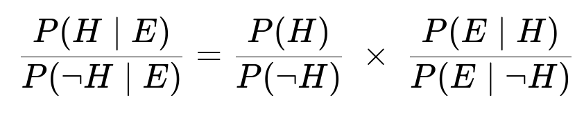
Let H be the event that a 1 is sent, and E be the event that a 1 is received. We use the odds form of Bayes’ theorem:

Substitute P(H) = 0.8, P(¬H) = 0.2, P(E|H) = 0.95, and P(E|¬H) = 1 − 0.99 = 0.01 into the formula. This yields
P(H|E)/P(¬H|E) = (0.8/0.2) * (0.95/0.01) = 4 * 95 = 380.
Therefore,
P(H|E) = 1 / (1 + 380) = 0.9974.
Comprehensive Explanation
Bayes’ theorem in its most familiar form is:
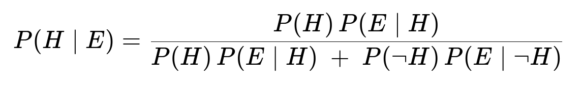
where
H is the hypothesis that a 1 was sent.
¬H is the hypothesis that a 0 was sent.
E is the evidence that a 1 was received.
P(H) is the prior probability that a 1 is sent (0.8).
P(¬H) is the prior probability that a 0 is sent (0.2).
P(E|H) is the likelihood of receiving a 1 given that a 1 was sent (0.95).
P(E|¬H) is the likelihood of receiving a 1 given that a 0 was sent (which is 1 − 0.99 = 0.01).
The odds form of Bayes’ theorem is:
We first compute the prior odds P(H)/P(¬H). Because we know P(H) = 0.8 and P(¬H) = 0.2, the prior odds is 0.8 / 0.2 = 4.
We then compute the Bayes factor, which is the ratio of likelihoods P(E|H)/P(E|¬H). The value of P(E|H) is 0.95, while P(E|¬H) is 0.01. Hence the Bayes factor is 0.95 / 0.01 = 95.
Multiply the prior odds by the Bayes factor: 4 * 95 = 380. This gives us the posterior odds P(H|E)/P(¬H|E).
To convert from odds to probability, we recall that if the odds are X, the corresponding probability for H is X / (1 + X). Hence:
P(H|E) = 380 / (1 + 380) = 380 / 381 = 0.9974 approximately.
This indicates that if we receive a 1, there is a very high posterior probability—about 99.74%—that the transmitted bit was indeed a 1.
The intuition behind this result is that sending a 1 is much more common than sending a 0 (80% vs. 20%), and our channel is very accurate at both sending 1 and 0 correctly (95% and 99% respectively). Together, these strong prior odds and good conditional accuracy lead to a large posterior probability favoring that the bit sent was 1 whenever we see a received 1.
What is the difference between the standard form of Bayes’ theorem and the odds form?
The standard form of Bayes’ theorem computes P(H|E) directly. It requires us to compute the marginal or normalizing constant in the denominator, which typically looks like:
P(H) P(E|H) + P(¬H) P(E|¬H).
The odds form, on the other hand, works with the ratio P(H|E)/P(¬H|E), which can sometimes simplify calculations. Instead of directly computing P(H|E), you compute how many times more likely H is than ¬H after seeing evidence E. Then you transform that odds ratio back into a probability if needed. The odds form is especially useful when dealing with sequential data updates or comparing multiple hypotheses in a straightforward multiplicative way.
How would the result change if the channel were extremely noisy?
If the channel became extremely noisy, that would translate into much lower values for P(E|H) and P(E|¬H) being closer together. For example, if receiving a 1 was equally likely whether a 1 or 0 was sent, then the likelihood ratio P(E|H)/P(E|¬H) would be near 1. In such a scenario, the evidence of receiving a 1 would not be very informative. As a result, P(H|E) would be closer to P(H), meaning we’d rely more on the prior probability and less on the evidence, because the evidence would not discriminate well between sending a 1 and sending a 0.
What if 1 and 0 were equally likely to be sent?
If P(H) = 0.5 and P(¬H) = 0.5, then the prior odds would be 1. In that case, the posterior odds would be determined solely by the likelihood ratio P(E|H)/P(E|¬H). If that ratio were still 0.95/0.01 = 95, then the posterior odds would be 95, and the posterior probability of sending a 1 given a received 1 would be 95/(1+95) = 0.987. This is still very high, but not as high as with the original 0.8 vs. 0.2 prior, because in the original question, the higher prior for sending a 1 (0.8) pushes the posterior probability up even more once a 1 is received.
How might we generalize this to transmissions with more than two symbols?
If we had multiple symbols (say digits 0 through 9) instead of just 0 and 1, we would extend Bayes’ theorem to multiple hypotheses:
Let H_i be the hypothesis that symbol i was sent.
Then the posterior probability of H_i given evidence E (that symbol j was received) would be proportional to P(H_i) P(E|H_i).
We would normalize over all possible symbols. Specifically,

The concept remains the same: each symbol has a prior probability, and we have a conditional probability of receiving symbol j given the transmitted symbol. In practice, you pick whichever symbol yields the highest posterior probability after normalizing.
Code snippet to verify in Python
p_H = 0.8  # Probability of sending 1
p_notH = 0.2  # Probability of sending 0

p_E_given_H = 0.95   # Probability of receiving 1 if 1 was sent
p_E_given_notH = 0.01  # Probability of receiving 1 if 0 was sent (1 - 0.99)

# Compute posterior using odds form
prior_odds = p_H / p_notH
likelihood_ratio = p_E_given_H / p_E_given_notH
posterior_odds = prior_odds * likelihood_ratio
posterior_probability = posterior_odds / (1 + posterior_odds)

print(posterior_probability)  # Should be ~0.9974
This quick check confirms that the posterior probability is indeed approximately 0.9974 when a 1 is received.
Below are additional follow-up questions
What if the estimated probabilities of sending 1 or 0 are inaccurate or change over time?
In many real-world communication scenarios, the true probability of sending 1 (the prior) could be different from the nominal 0.8. It might vary over time or might have been incorrectly estimated. Suppose initially you believe P(H)=0.8, but over time you discover it actually fluctuates (e.g., some time windows send more 1's than others).
When you have uncertain or dynamic priors:
You may model the prior probability of sending a 1 as a random variable itself and update it with data. This approach is called hierarchical Bayesian modeling or sometimes empirical Bayes if you estimate the prior from observed transmissions.
If your system detects changing conditions (e.g., different time of day or different segments of data), you might adapt P(H) in real time, using, for example, a moving average of how many 1’s vs. 0’s you’ve actually seen transmitted lately.
A major pitfall is that if your prior is significantly off (say you assume 0.8 but it’s really 0.5), then your posterior inference can be quite misleading. Always verify or recalibrate your priors with empirical data whenever possible.
How can we handle scenarios where P(E|H) and P(E|¬H) themselves might be uncertain?
In practice, channel reliability parameters (e.g., 0.95 for receiving a 1 when sending a 1, and 0.99 for receiving a 0 when sending a 0) are themselves estimates. If we are not absolutely sure about these values, we need to:
Collect a training dataset of sent bits and received bits to estimate these conditional probabilities. For instance, you might find that your 0.95 estimate is really around 0.92 in practice, which can significantly affect your posterior.
Consider a Bayesian approach where you treat P(E|H) and P(E|¬H) as random variables with prior distributions (e.g., Beta distributions for probabilities). As you collect data, you update the posterior over these probabilities. This yields a posterior distribution of P(H|E) that incorporates uncertainty about the channel parameters.
Periodically re-estimate or re-check these probabilities if the transmission environment changes (e.g., interference, different hardware, or changing power levels).
What happens if the cost of misclassifying a received bit is not the same in both directions?
Often in real applications, confusing a 1 for a 0 might be more or less costly than confusing a 0 for a 1. For instance, if a 1 signals a critical alert, you might want to minimize false negatives more than false positives. In such cases:
The standard Bayes’ decision rule for “choose H if P(H|E) > 0.5” might not be optimal. Instead, you might incorporate a loss function or cost matrix, so you would choose the hypothesis that minimizes expected cost.
A typical approach is to compare P(H|E) * (cost of wrongly deciding ¬H) against P(¬H|E) * (cost of wrongly deciding H). You pick the hypothesis with the lower expected cost. This is known as Bayesian decision theory.
Edge cases arise if one cost dwarfs the other: for example, if the cost of failing to detect a 1 is extremely high, you might set a very low threshold for deciding 1, which can increase false positives but reduce the risk of missing true 1’s.
How does noise correlation between successive transmitted bits affect the inference?
The derivation usually assumes each bit is transmitted independently with its own probability of error. However, in many physical channels, noise can be correlated across time (e.g., burst errors). This correlation complicates the analysis because:
The probability of receiving a 1 at time t could depend on what happened at time t−1, t−2, etc.
A straightforward single-bit application of Bayes’ theorem ignores these correlations. A more accurate model might need a Hidden Markov Model (HMM) or a dynamic Bayesian network, incorporating the transition probabilities of bits and the correlated noise.
In an HMM approach, you would perform forward-backward algorithms to compute the posterior probability of each transmitted bit sequence given the entire sequence of received bits. This is more computationally intensive but yields better results when errors occur in bursts.
What if there is a possibility of no bit being sent at all (e.g., missing data)?
Sometimes real systems might experience packet drops or partial transmissions leading to no data received in a time slot:
You can model a third event N: “No bit was sent or the signal was lost.” Then you have three hypotheses: H for “1 was sent,” ¬H for “0 was sent,” and N for “nothing was sent.” Each has a prior probability, and you define P(E|N), the probability of receiving a 1 if indeed nothing was sent (perhaps representing stray noise).
Bayes’ theorem must then be expanded over all three hypotheses. For instance, the posterior for H would be proportional to P(H) * P(E|H), but you must normalize by P(H)*P(E|H) + P(¬H)*P(E|¬H) + P(N)*P(E|N).
A subtle pitfall is if you incorrectly ignore the possibility that the bit never arrived, you might drastically inflate or deflate the posterior for H when you see E=1.
How does one approach bit errors in a more complex channel coding scheme?
In modern communication systems, bits are often encoded (e.g., with CRC checks, forward error correction) to reduce net error rates:
Instead of calculating P(H|E) at the bit level, the system typically tries to decode entire codewords. For instance, a convolutional or block code might be used, and the receiver uses a decoding algorithm (like Viterbi) that internally uses likelihoods for sequences of bits.
Bayes’ theorem is still the conceptual foundation: the decoder constructs or approximates the posterior probability of each possible transmitted codeword.
Once the codeword is decided, the final bit decisions are derived from the codeword that maximizes posterior probability. This often leads to a much lower bit error rate compared to decoding bits independently.
Could we leverage Bayes’ theorem for real-time error correction?
Yes, you can do iterative or sequential Bayesian updating if data arrives in small chunks or streaming fashion:
Start with an initial prior P(H). After receiving each bit (or block), update to the posterior using the evidence. That posterior becomes the new prior for the next bit. This is helpful if you suspect the channel conditions or the prior probabilities shift over time.
This can also integrate seamlessly with real-time error correction algorithms, effectively giving you a dynamic estimate of the channel reliability (i.e., your updated P(E|H) and P(E|¬H)) and your prior for bits.
What if we have multi-level signals, but we threshold them to 0/1 in hardware?
In many practical systems, the raw signal is a continuous amplitude or voltage. A hardware comparator threshold might then produce 0 or 1:
The probabilities P(E=1|H) or P(E=1|¬H) reflect the distribution of the continuous signal around the threshold. If the signal-to-noise ratio is high, these probabilities will be close to 1 or 0. If the SNR is poor, both probabilities might drift toward 0.5.
A pitfall is if the threshold is miscalibrated. Then even a high SNR system can produce substantial errors, because the distribution for 1 might overlap significantly with the threshold. Recalibrating the threshold or modeling the distribution of signal values more precisely can reduce error rates.
