
ML Interview Q Series: Demystifying Logistic Regression Coefficients: Understanding Log-Odds and Odds Ratios

📚 Browse the full ML Interview series here.
The Interpretation of Logistic Regression Coefficient
Understanding the interpretation of logistic regression coefficients can be tricky because logistic regression uses the log-odds (rather than a straight linear function) to connect features to the probability of a binary outcome.
What does that mean
Logistic regression turns each feature’s impact into a change in log-odds rather than a direct change in probability. The log-odds is just a mathematical way to keep the predicted probability between 0 and 1. So instead of saying “increasing a feature by 1 raises the probability by X,” we say “it raises the log-odds by X.” Exponentiating that amount tells you how many times the odds (ratio of probability of success vs. failure) change. This extra step makes the relationship easier for the math to handle but less direct to interpret than a simple linear model.
What exactly the term 'log-odds' means. tell me with very simple example
Log-odds is simply the natural logarithm of the “odds.” The odds of an event is the ratio of the probability that the event happens to the probability it does not happen. For example:
If the probability of raining is (0.75), then:

Why do we use log-odds in logistic regression?
Log-odds let us keep the model’s output (the probability) within 0 and 1. If we used a linear function directly for probability, we could end up with impossible values below 0 or above 1. By working with log-odds, the final probability always stays valid while still allowing a straight-line relationship in the log-odds space.
Could you provide a short illustrative scenario?
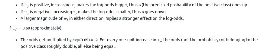
Imagine you’re predicting if someone passes an exam. The model might learn that each extra hour of study multiplies the odds of passing by, say, 2. If you start with 1-to-1 odds (50% chance to pass), one more hour of study turns that into 2-to-1 odds (about 67% chance to pass). Another hour would make it 4-to-1 odds (80% chance), and so on. The log-odds are just the natural log of those multiples, allowing the model to treat them as if they increase by a constant amount when you add one more hour.
Below is a deeply detailed explanation of how these coefficients work and how to interpret them in various contexts, along with illustrative code and potential questions an interviewer might ask you to test your depth of knowledge.
The Core Idea of Log-Odds
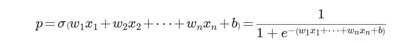
A logistic regression model predicts the probability of the positive (or "1") class, denoted as (p). Instead of modeling (p) directly in a linear form, logistic regression models the log-odds (also referred to as the logit) of (p). The log-odds is:

Probability Connection
Even though the model “internally” deals with log-odds, it ultimately outputs a probability. The probability (p) is recovered by applying the logistic (sigmoid) function:
From the above, the coefficients still fundamentally “live” in log-odds space. This leads to a particular interpretation for each coefficient.
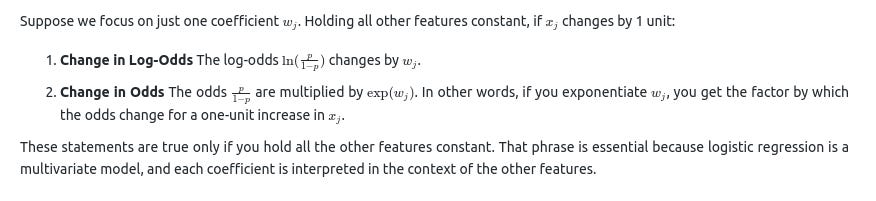
Interpreting a Single Coefficient
Example Interpretation in Plain Words
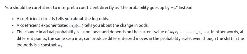
Important Nuance: Probability vs. Odds
Code Example Demonstrating Interpretation
import numpy as np
from sklearn.linear_model import LogisticRegression

# Simple dataset with one feature
X = np.array([[1.0], [2.0], [3.0], [4.0], [5.0]])
y = np.array([0, 0, 0, 1, 1])

# Fit logistic regression
model = LogisticRegression()
model.fit(X, y)

# Extract the single coefficient and intercept
coef = model.coef_[0][0]
intercept = model.intercept_[0]

# Print them
print("Coefficient (w):", coef)
print("Intercept (b):", intercept)

# Exponentiate the coefficient to see the factor change in odds
odds_factor = np.exp(coef)
print("Odds are multiplied by:", odds_factor, "for a 1-unit increase in X")
In the above:
coefis (w).interceptis (b).`odds_factor = np.exp(w)) is the multiplier for the odds per one-unit increase in (X).
Why Log-Odds?
By using log-odds, logistic regression ensures the output probability remains between 0 and 1. If we let the model’s linear combination directly represent probability, we could get invalid probabilities below 0 or above 1. The logistic function keeps predictions in a valid probability range but preserves a linear relationship in log-odds space.
Impact of Feature Scaling on Interpretation
If one feature is measured on a large scale (e.g., annual income in dollars), a coefficient for that feature may appear very small. Another feature on a smaller scale (e.g., number of cars) might have a larger coefficient. This does not necessarily mean the second feature is more “important.” It just means a one-unit increase in the second feature can be more influential in log-odds terms than a one-unit (one dollar) increase in the first.
Because of this, many practitioners standardize or normalize features before fitting logistic regression. After standardization, a one-unit increase becomes “one standard deviation increase,” which can make comparing coefficient magnitudes more intuitive.
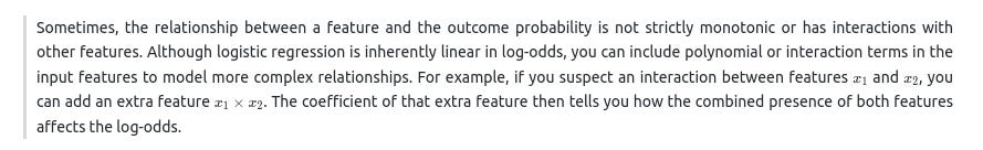
Interactions and Nonlinearity

Regularization and Coefficient Shrinkage
In many software implementations (e.g., scikit-learn’s default
LogisticRegression), a regularization penalty is applied (often L2). This penalty shrinks coefficients toward zero to reduce overfitting. While it doesn’t change the fundamental interpretation of the coefficients, it affects their final magnitudes. With strong regularization, you might see smaller absolute coefficient values, indicating that the model is forced to keep the log-odds changes conservative.Holding Other Variables Constant
One subtle but crucial assumption in interpreting logistic regression coefficients is the phrase “holding all other variables constant.” In a real dataset, features might be correlated or might change together in practice. Strictly speaking, the interpretation is always made in a partial sense: “For the same values of all other features, an increase of one unit in feature (x_j) changes the log-odds by (w_j).”
Challenges in Interpretation
Multicollinearity: When features are highly correlated, the model’s coefficients can become unstable. That can lead to large, counterintuitive coefficients or large changes in coefficients if a single feature is removed or added.
Non-Stationarity: If the relationship between feature values and the outcome changes over time or across different subgroups, the same coefficient might not hold uniformly across all samples.
Categorical Variables: For categorical variables (e.g., “Red”, “Blue”, “Green”), we typically encode them as dummy variables. Each category’s coefficient will be relative to the “baseline” (the omitted category).
Illustrating a Multi-Feature Example
Below is a quick demonstration with multiple features:
import numpy as np
from sklearn.linear_model import LogisticRegression

# Synthetic dataset with two features
# Let's say these features represent [hours_slept, coffee_cups]
X = np.array([
    [7.0, 2],
    [6.5, 1],
    [5.0, 3],
    [8.0, 0],
    [7.5, 1],
    [4.0, 4],
    [5.5, 2],
    [6.0, 2]
])
# Suppose 1 = "productive day", 0 = "not productive day"
y = np.array([1, 1, 0, 1, 1, 0, 0, 0])

model = LogisticRegression()
model.fit(X, y)

print("Coefficients:", model.coef_)
print("Intercept:", model.intercept_)

odds_factors = np.exp(model.coef_)
print("Odds change factors (exp of coefficients):", odds_factors)
Interpreting the first coefficient (associated with hours slept):
If it’s positive, more sleep increases the log-odds of productivity.
The exponentiated coefficient tells you how many times the odds of being productive multiply for each additional hour of sleep.
Interpreting the second coefficient (associated with coffee cups):
A positive coefficient suggests more coffee cups increase the log-odds of a productive day.
If negative, more coffee cups reduce the log-odds of productivity (perhaps from overstimulation or other confounders).
Again, all interpretations hold other features constant. In real life, you can’t always perfectly isolate one feature’s effect, but that’s how logistic regression mathematically interprets them.
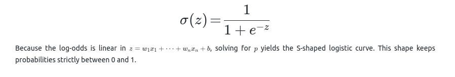
Why is This Called a “Logistic” Regression?
The function that maps a linear combination of features to a probability is called the logistic (or sigmoid) function:
Common Follow-Up Questions About Interpretation
Below are typical questions an interviewer might ask if they feel your explanation is incomplete or if they want to probe further.
Can you give a more intuitive example of log-odds in everyday language?
If you ask this question:

How does interpreting coefficients differ between linear and logistic regression?
If you ask this question:
In linear regression, a coefficient directly states how much the outcome (e.g., house price) changes with a one-unit change in a predictor, holding others constant.
In logistic regression, a coefficient states how the log-odds of the positive event changes with a one-unit change in that predictor. Because of the logistic transform, this translates to a multiplicative change in the odds. You do not say “the probability goes up by (w)”—rather, “the log-odds goes up by (w), so the odds multiply by exp(w).”

What happens to coefficient interpretation when using regularization?
If you ask this question:
Regularization (especially L2) shrinks the magnitude of coefficients toward zero to avoid overfitting. The interpretation remains the same in a technical sense, but each (w_j) might be smaller (or closer to zero) than if you fit the model without regularization. Practically, it means the model does not rely too heavily on any single feature unless that feature truly has a strong and consistent effect. Interpretation in terms of multiplying the odds by exp(w_j) for a one-unit increase is still valid—just be aware that the magnitude might be smaller because of the penalty.
How do correlated features affect coefficient interpretation?

How can I confidently say which feature is the most important?
If you ask this question:
Importance can be measured in multiple ways:
By the absolute size of the coefficient in log-odds space (larger absolute values mean a stronger effect on log-odds).
By the factor change in odds exp(w_j).
By how removing a feature affects predictive performance (feature ablation).
By computing standardized coefficients (especially if you standardize all features).
By partial dependence plots or other advanced interpretability methods that show how predicted probability changes as you vary a feature over its range.
Each method highlights a different notion of “importance.” For purely interpretive tasks, exp(w_j) can be quite direct. But for predictive tasks, sometimes simply measuring the drop in predictive power if you shuffle that feature or remove it from the model can be more revealing.
If I only have categorical features, is interpretation still the same?
If you ask this question:
Yes, but with a small nuance. A categorical feature with multiple categories is typically turned into dummy variables (one-hot encoding). Each dummy variable might be 1 for that category and 0 otherwise. The “baseline” category is the one that does not get a dummy variable. Each coefficient tells you how belonging to that category (vs. the baseline category) changes the log-odds. The same log-odds interpretation applies, except “a one-unit increase” for a dummy variable means “switching from not being in that category to being in that category.”
What if the model has trouble converging and I don’t trust the coefficients?
If you ask this question:
Difficult convergence might imply:
High multicollinearity among features.
Extremely large or small feature scales.
Overly strong or overly weak regularization settings.
Insufficient data or ill-posed classification tasks.
Cleaning the dataset, removing or merging redundant features, standardizing numeric features, and adjusting your regularization parameter (the C parameter in scikit-learn) can all help stabilize the solution. Once the model converges properly, the coefficient interpretation reverts to the standard log-odds interpretation.
How do I explain logistic regression coefficients to a non-technical stakeholder?
If you ask this question:
You can say something like: “We have a model that predicts whether something is likely to happen or not. Each feature has a number (coefficient). If that number is positive, it means that having more of this feature generally increases the likelihood of the outcome. If it is negative, more of that feature decreases the likelihood of the outcome. The size of the number tells us how strong that effect is, but because it’s on a log scale, we often look at exp(w_j) to see how much the odds are multiplied. For example, if (exp(w_j) = 1.5), it means that each extra unit of that feature multiplies the odds of the outcome by 1.5, holding other features the same.”
Wrap-Up of Interpretation
A logistic regression coefficient says: “For a one-unit increase in the feature (x_j), the log-odds of the target being 1 (instead of 0) increase by (w_j).” Equivalently, you can exponentiate that coefficient (exp(w_j)) to discover how much the odds multiply. While that is the crux, the real world adds layers of complexity—correlations, feature scaling, regularization, and domain nuances. But the fundamental interpretation remains tied to log-odds and their exponential relationship to odds.
This knowledge is critical in interviews, where you may be asked to justify how logistic regression arrives at its predictions and how exactly each coefficient translates into an effect on the modeled probability. Having a solid grasp of log-odds, odds, and probability transformations is essential to demonstrate your depth of understanding.