
ML Interview Q Series: Deriving Conditional Binomial Distribution from a Joint Probability Mass Function.

Browse all the Probability Interview Questions here.
Question
Let
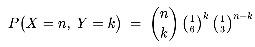
for k = 0, 1, …, n and n = 1, 2, … be the joint probability mass function of the random variables X and Y. What is the conditional distribution of Y given that X = n?
Short Compact solution
Summing over k from 0 to n in the joint PMF shows that
P(X = n) = (1/2)^n.
Hence X is a geometric random variable with parameter 1/2. Then
P(Y = k | X = n) = ( (n choose k) (1/6)^k (1/3)^(n-k) ) / (1/6 + 1/3)^n
which simplifies to
Comprehensive Explanation
Deriving the marginal distribution of X
Definition of the joint PMF We are given: P(X=n, Y=k) = (n choose k)(1/6)^k (1/3)^(n-k), valid for k = 0, 1, …, n and n = 1, 2, ….
Sum out Y to find P(X=n) We compute P(X=n) by summing over all possible values of k: P(X=n) = sum over k=0..n of (n choose k)(1/6)^k (1/3)^(n-k).
Notice that 1/6 + 1/3 = 1/2. Hence by the binomial expansion: sum over k=0..n of (n choose k)(1/6)^k (1/3)^(n-k) = (1/2)^n.
Therefore: P(X=n) = (1/2)^n.
This is exactly the form of a geometric distribution on the positive integers if we interpret n as the nth trial on which something happens. Indeed, one can check carefully that X takes values n=1,2,… with P(X=n) = (1/2)^n, which is consistent with the parameter of a geometric distribution being 1/2 (though note the slight shift in indexing depending on whether a geometric random variable is defined to start at n=1 or n=0, but here it starts from n=1).
Deriving the conditional distribution P(Y = k | X = n)
Definition of conditional probability By definition, P(Y=k | X=n) = P(X=n, Y=k) / P(X=n).
From the problem statement, P(X=n, Y=k) = (n choose k)(1/6)^k (1/3)^(n-k).
From the marginal distribution, P(X=n) = (1/2)^n.
Therefore,
P(Y=k | X=n) = [ (n choose k)(1/6)^k (1/3)^(n-k) ] / (1/2)^n.
Algebraic simplification We factor out (1/2)^n = (1/6 + 1/3)^n from the numerator to see:
(1/6)^k (1/3)^(n-k) = (1 / 6^k)(1 / 3^(n-k)) = 1 / (2^k 3^n).
Dividing by (1/2)^n is equivalent to multiplying by 2^n. Thus the ratio becomes:
(n choose k) [ 2^n / (2^k 3^n ) ] = (n choose k) [ 2^(n-k) / 3^n ].
A more recognizable binomial form appears if we rewrite 2^(n-k)/3^n as (1/3)^k (2/3)^(n-k). Indeed:
(1/3)^k (2/3)^(n-k) = (2^(n-k) / 3^(n-k)) (1 / 3^k) = 2^(n-k) / 3^n.
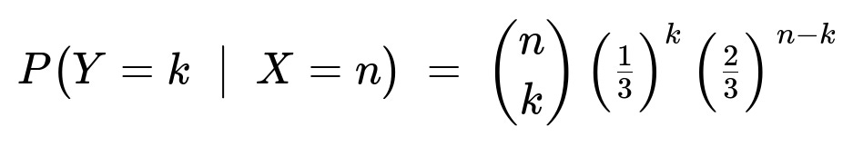
Hence the conditional distribution is:
for k = 0, 1, …, n. This is exactly the PMF of a Binomial(n, 1/3) distribution.
Interpretation
Once X = n has occurred, Y behaves like the number of “successes” out of n Bernoulli trials, with success probability 1/3.
In other words, conditioned on X = n, Y ~ Binomial(n, 1/3).
Intuitively, within each “trial” that eventually contributed to X=n, the chance that Y increments is (1/6)/(1/2) = 1/3, because 1/6 is the factor associated with one event type and 1/3 is associated with another event type, and they total 1/2 in the denominator.
Potential Follow-up Questions
Why is X geometric with parameter 1/2?
When we marginalize out Y, we get: P(X=n) = (1/2)^n. One can verify that summing ( (n choose k)(1/6)^k(1/3)^(n-k) ) from k=0 to n yields (1/2)^n, which is the probability mass function of a geometric random variable (with support n=1,2,…) having parameter 1/2. The standard geometric distribution can be parameterized so that P(X=n) = (1 - p)^(n-1) p, or in a form starting at n=1 with P(X=n) = (1-p)^n p/(1-p). In this problem, the final simplified form effectively identifies p=1/2 under an appropriate indexing. Ensuring the details match depends on precisely how one defines the support (starting at 1 or 0), but the core fact is that each n is downweighted by (1/2)^n in the same ratio that a geometric distribution would produce.
Could we have deduced directly that Y|X=n is Binomial(n, 1/3)?
Yes. Notice that:
The joint PMF is the product of a combinatorial factor (n choose k) and two probability “weights,” 1/6 and 1/3.
If we define the probability of “success” in each trial as the ratio (1/6) / [(1/6)+(1/3)] = 1/3, we see that the conditional distribution of k out of n “successes” in that sense is indeed Binomial(n, 1/3).
Are X and Y independent?
They are not independent. If you observe a particular value of X=n, that restricts the possible range for Y to 0..n. So Y depends on X, and the unconditional distribution of Y is not the same as Y’s distribution given X=n. Indeed, marginally, Y has a distribution that can be computed by summing P(X=n, Y=k) over n, but Y’s value is constrained by X.
What happens if we try small values of n for verification?
Take n=2. Then the possible values of k are 0, 1, 2:
Joint probabilities: P(X=2, Y=0) = (2 choose 0)(1/6)^0(1/3)^2 = (1)(1)(1/9) = 1/9 P(X=2, Y=1) = (2 choose 1)(1/6)^1(1/3)^1 = 2 * (1/6)(1/3) = 2/18 = 1/9 P(X=2, Y=2) = (2 choose 2)(1/6)^2(1/3)^0 = 1 * (1/36)(1) = 1/36
Summing: 1/9 + 1/9 + 1/36 = 2/9 + 1/36 = 8/36 + 1/36 = 9/36 = 1/4 = (1/2)^2, as expected for P(X=2).
Conditional probabilities: P(Y=0 | X=2) = (1/9) / (1/4) = 4/9 P(Y=1 | X=2) = (1/9) / (1/4) = 4/9 P(Y=2 | X=2) = (1/36) / (1/4) = 1/9
Checking the binomial form Binomial(2, 1/3): (2 choose 0)(1/3)^0(2/3)^2 = 1*(1)(4/9) = 4/9 (2 choose 1)(1/3)^1(2/3)^1 = 2(1/3)(2/3) = 4/9 (2 choose 2)(1/3)^2(2/3)^0 = 1(1/9)*1 = 1/9
Matches perfectly.
This consistency check confirms that our conditional distribution is correct.
Below are additional follow-up questions
Could the random variable X have started from 0 instead of 1, and how would that change the interpretation of the distribution?
One subtlety in defining geometric distributions is whether we allow X = 0 or start X at 1. In the problem, X takes positive integer values 1, 2, 3, …, with P(X=n) = (1/2)^n. If one instead considered a version of X that starts at 0 (i.e., X=0,1,2,3,…), the parameters and formula would typically shift:
For a geometric distribution starting at 0, the PMF is often given by P(X=x) = (1 – p)^{x} p for x = 0, 1, 2, …
In this problem, with parameter p=1/2, that would become P(X=x) = (1/2)(1/2)^{x} = (1/2)^{x+1}.
Hence, if X had included 0 in its support, the joint probability P(X=0, Y=0) would need consideration. But from the problem statement, there is no P(X=0) because n runs from 1 to infinity, and in the combinatorial expression (n choose k), n=0 and k=0 is typically a separate case. Thus it is consistent with a geometric distribution that starts at 1.
In practical terms, whether the distribution starts at 0 or 1 can matter if we are modeling the number of “trials up to and including the first success” versus “the number of failures before the first success.” For the problem at hand, we see that X must be at least 1, so the chosen parameterization is consistent with many standard references where Geometric distributions are enumerated from n=1,2,3,…
Does the joint distribution necessarily sum to 1 across all valid (n, k) pairs, and why is that important?
Yes, the sum of P(X=n, Y=k) over n = 1 to infinity and k = 0 to n must equal 1 for it to be a valid joint PMF. Formally,
sum_{n=1 to infinity} sum_{k=0 to n} (n choose k) (1/6)^k (1/3)^(n-k) = sum_{n=1 to infinity} (1/2)^n.
The binomial sum over k for each fixed n gives (1/6 + 1/3)^n = (1/2)^n. Then we sum (1/2)^n from n=1 to infinity, which is (1/2) / (1 - 1/2) = 1. This confirms the total probability is 1.
If this normalization did not hold, the distribution would be invalid. In real-world applications, failing to verify that the total probability sums (or integrates) to 1 is a common pitfall, indicating potential errors in modeling or parameter constraints.
How could we interpret Y as a “partial” count within the geometric structure of X?
Conceptually, X can be seen as the total number of “trials” completed until a certain stopping condition. Then Y is the number of “type-1 successes” within those X trials. Specifically:
Each trial can result in: – “Type-1 success” (probability 1/6). – “Type-2 success” (probability 1/3). – No success or unmodeled outcome (in a typical geometric setting) might be accounted for by the difference, but here the total probability for a “success” of either type is (1/6 + 1/3) = 1/2, leading to the stopping event after exactly one of these half-chance “successes” each trial in a more generalized geometric sense.
Y effectively tracks how many times we observe the type-1 event across those n trials. Once the nth trial completes the process, the total is locked in. That is why Y ≤ n and Y is binomially distributed given X=n.
If we define Z = X – Y, what can we say about Z and its distribution?
With X = n and Y = k, then Z = n – k. Intuitively, Z counts the number of “type-2 successes” (probability 1/3 for each trial’s “success” event) within the n trials, whereas Y counts the “type-1 successes” (probability 1/6 for each trial’s “success” event). Once we condition on having X = n total trials (that is, n total “success” events in the sense that each trial produced either type-1 or type-2 success), we know Y+k+Z = n with Y = k, Z = n–k.
Hence, conditioned on X = n, Z also follows a Binomial(n, 2/3) if we think of “type-2 success probability” as (1/3) / (1/6 + 1/3) = 2/3. In other words,
Y ~ Binomial(n, 1/3),
Z ~ Binomial(n, 2/3),
Y + Z = n.
In fact, Y and Z are perfectly determined by each other once n is known, since Y = n – Z. Taken together, Y and Z cannot vary independently once X=n is fixed.
If we define W = Y / X, is W independent of X, and how can we think about its distribution?
W = Y / X is the fraction of type-1 successes among the total. Since Y | X=n ~ Binomial(n, 1/3), the fraction Y / X is basically (1/3) plus some random deviation that depends on n. For large n, by the Law of Large Numbers, Y / n will likely be near 1/3. But W is not strictly independent of X:
If X is small, Y can only take a small set of integer values, so W can take only discrete fractions (like 0/1, 1/1, …).
If X is large, Y / X has more possible fractional values and is likely to center around 1/3.
Thus, X and W are not independent. Formally, independence would require that knowing X=n provides no information about W, but obviously if n=1, W is either 0 or 1, whereas if n=10, W has multiple possibilities.
How might we apply such a model in real-world scenarios, and what pitfalls could occur if assumptions are incorrect?
In real-world applications, one might view X as the total number of attempts up to some “critical event,” and Y as the number of times a sub-event occurs among those attempts. For instance, imagine a scenario in health data where X is the number of patient visits before a certain threshold is reached, and Y is how many times a specific outcome was recorded among those visits.
Pitfalls and subtle issues include:
Overlooking that X might not truly follow a geometric distribution if the probability of a “success” changes over time (e.g., non-constant hazard rates).
Failing to validate that Y given X is genuinely binomial. In practice, the probability of a sub-event may vary with each trial, so the binomial assumption might be violated.
Confounding factors: Additional variables might influence both the total count X and the fraction Y/X, invalidating the straightforward geometric-binomial separation.
If these assumptions break, the model’s predictions and inferences (e.g., confidence intervals around Y for a given X) could be systematically biased.
How would we perform maximum likelihood estimation (MLE) if we had empirical data for X and Y, and what are potential pitfalls?
In principle, if you have a dataset {(x_i, y_i)} of observations, you can write down the likelihood function:
L(p_1, p_2) = Product over i of [ (x_i choose y_i) (p_1)^{y_i} (p_2)^{x_i - y_i} ] * (p_1 + p_2)^{x_i},
where p_1 + p_2 is the probability that each trial yields a “success” (contributing to X). However, in the original statement, p_1=1/6 and p_2=1/3 were presumably known. If these parameters were unknown, you would need to ensure:
p_1 + p_2 = p < 1 (for the geometric mechanism to make sense), with p being the chance of stopping each trial.
Y_i ≤ X_i for each data point.
A common pitfall: If the data is small, or if certain values of X are underrepresented, the MLE might lead to degenerate solutions (like pushing p_2 too large or too small). Another subtlety is that standard closed-form MLE expressions might not exist for all parameter combinations, so numerical optimization could be required. One must also verify that the estimated parameters keep p_1 + p_2 < 1, or else the “geometric-like” assumption fails.
How do we simulate from this joint distribution, and what constraints must we respect?
To simulate (X, Y):
Simulate X from its geometric distribution with parameter p=1/2, i.e., generate X=n with probability (1/2)^n (n≥1).
Given that X=n, simulate Y from Binomial(n, 1/3).
This yields valid (n, y) pairs with Y ≤ n. A key constraint is that Y can never exceed X. In practice, one must ensure the random generation respects that Y is generated after X is known. Attempting to draw X and Y independently without the binomial conditioning would lead to many invalid draws (cases where Y>n or other misalignment).
If you skip the condition Y ≤ X or ignore it in code, you would risk generating impossible outcomes, which is a common pitfall in naive simulation approaches.
If we change 1/6 and 1/3 to other values, do we still preserve the binomial form for Y|X?
Yes, as long as the joint probability can be factored in the form
(n choose k) (p_1)^k (p_2)^{n-k},
where p_1 + p_2 is the sum over all event types that define “success.” Then the marginal distribution for X would be (p_1 + p_2)^n times the probability that these successes continue for n trials. As long as there is a consistent ratio that yields a geometric distribution in X (the sum p_1 + p_2 < 1 to ensure a valid geometric process, or equals something that normalizes with the rest of the process if X can go infinite), the conditional distribution for Y given X=n will remain Binomial(n, p_1 / (p_1 + p_2)).
The key structural property is that Y arises from one particular outcome type among the total “successes” counted by X. That leads to a binomial conditional structure whenever the probability for that outcome type is constant on each trial. If p_1 + p_2 changes, or if p_1 and p_2 vary with each trial, then that structure no longer applies.