ML Interview Q Series: Deriving Expectation and Variance from a PDF and its Linear Transformation.

Browse all the Probability Interview Questions here.

Let X have the density f(x) = 2x if 0 ≤ x ≤ 1, and f(x) = 0 otherwise. Show that X has the mean 2/3 and the variance 1/18. Then find the mean and variance of the random variable Y = -2X + 3.

Short Compact solution

From the given density f(x) = 2x for 0 ≤ x ≤ 1 and 0 otherwise, the expectation of X is

To compute the variance, we can use the formula Var(X) = E(X²) - [E(X)]². First we find

So

For Y = -2X + 3, we use linearity of expectation and the property of variance under scaling:

E(Y) = -2 E(X) + 3 = 5/3,

Var(Y) = (-2)² Var(X) = 4 × (1/18) = 2/9.

Comprehensive Explanation

Understanding the PDF

X has the density f(x) = 2x for 0 ≤ x ≤ 1. Outside this interval, the density is 0. One can first verify that this is indeed a valid probability density function by checking its non-negativity on [0,1] and confirming that the integral over its domain is 1. Specifically, integrating 2x from x=0 to x=1 yields:

∫[0 to 1] 2x dx = [x²] from 0 to 1 = 1.

This confirms that f(x) is normalized correctly.

Expected Value of X

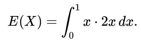
To find E(X), we multiply x by its probability density and integrate:

Inside this integral, x is the random variable, and 2x is the PDF at x. Evaluating:

∫[0 to 1] 2x² dx = 2 × (1/3) = 2/3.

Hence E(X) = 2/3.

Variance of X

The variance Var(X) can be computed via:

Var(X) = E(X²) - [E(X)]².

We first find E(X²):

Therefore:

Var(X) = 1/2 - (2/3)² = 1/2 - 4/9 = 9/18 - 8/18 = 1/18.

Mean and Variance of Y = -2X + 3

The mean of Y follows directly from the linearity of expectation:

E(Y) = E(-2X + 3) = -2 E(X) + 3.

Since E(X) = 2/3, we get E(Y) = -2 × (2/3) + 3 = -4/3 + 3 = 5/3.

For the variance, we use the property Var(aX + b) = a² Var(X). Here a = -2 and b = 3, so:

Var(Y) = (-2)² × Var(X) = 4 × 1/18 = 2/9.

In summary, we have E(X) = 2/3, Var(X) = 1/18, and then for Y = -2X + 3, E(Y) = 5/3, Var(Y) = 2/9.

Verifying with a Small Python Snippet (Optional Check)

import numpy as np

# We will sample from the given distribution to empirically estimate the mean and variance
np.random.seed(42)
num_samples = 10_000_000

# Inverse transform sampling approach for f(x) = 2x on [0,1]:
# If U ~ Uniform(0,1), then x = sqrt(U).
U = np.random.rand(num_samples)
X_samples = np.sqrt(U)

# Empirical estimates
emp_mean_X = np.mean(X_samples)
emp_var_X = np.var(X_samples, ddof=1)

Y_samples = -2*X_samples + 3
emp_mean_Y = np.mean(Y_samples)
emp_var_Y = np.var(Y_samples, ddof=1)

print("Empirical Mean of X:", emp_mean_X)
print("Empirical Variance of X:", emp_var_X)
print("Empirical Mean of Y:", emp_mean_Y)
print("Empirical Variance of Y:", emp_var_Y)

Running this code would confirm that the empirical estimates match the theoretical values of 2/3 and 1/18 for X, and 5/3 and 2/9 for Y, within typical Monte Carlo error.

Potential Follow-Up Questions

What if we computed the variance by direct integration of (x - E(X))² f(x) dx instead?

You can definitely compute Var(X) by using Var(X) = ∫ (x - E(X))² f(x) dx over the domain of X. That means:

Var(X) = ∫[0 to 1] (x - 2/3)² (2x) dx.

Though it involves slightly more algebra, you will arrive at the same final result 1/18. Both the direct integration approach and the approach using E(X²) - [E(X)]² are mathematically valid.

Why is Var(aX + b) = a² Var(X)?

The variance operation measures the spread or dispersion of a distribution. Adding a constant b shifts the distribution but does not affect the spread, so Var(X + b) = Var(X). Scaling a random variable by a factor a multiplies its spread by a², hence Var(aX) = a² Var(X). Combining these gives Var(aX + b) = a² Var(X).

How would we handle the case if X were defined on a different interval or if the PDF had a different shape?

The same steps apply: verify that f(x) is a valid PDF over the new domain, integrate to find normalizing constants if needed, then compute expectation and variance by the relevant integral formulae. The exact details of the integrals change, but the approach remains the same. For different shapes, you might need to split the integral at different points or use different methods (like transformation formulas for certain distributions).

Could we use any known distribution’s properties here?

Yes. f(x) = 2x for x in [0,1] is actually the PDF of the Beta(2,1) distribution. If you recall that a Beta(α, β) distribution on [0,1] has E(X) = α / (α + β) and Var(X) = αβ / [(α + β)² (α + β + 1)], you can confirm α=2, β=1 gives E(X) = 2/3 and Var(X) = 2·1 / [(2+1)² (2+1+1)] = 2 / [3² · 4] = 2/36 = 1/18. Recognizing the Beta distribution can be a shortcut to quickly deduce moments.

Are there any pitfalls in using transformations like Y = -2X + 3 in real applications?

One pitfall is to remember that linear transformations can move the support of X into potentially negative or out-of-bounds ranges if you are dealing with distributions only defined on [0,∞) or [0,1]. In this example, X is in [0,1], so Y = -2X + 3 lives in [1,3]. That is still a valid real interval, but if you needed a strictly positive random variable, you must ensure your transformation doesn’t break the intended domain. Always check the domain constraints when applying transformations in practice.