
ML Interview Q Series: Deriving Geometric Random Variable Expectation Using Geometric Series Differentiation.

Browse all the Probability Interview Questions here.
Explain how one can derive the expected value of a geometric random variable.
Comprehensive Explanation
Definition and Setup
A geometric random variable X models the number of Bernoulli trials that occur until the very first success is observed. Each trial has a success probability p and is independent of the others. The probability mass function (PMF) can be written as:

This version of the geometric random variable specifically counts the trial on which the first success happens.
Key Idea for the Expectation
The expected value E[X] is computed by the infinite series:

In order to evaluate this sum, one can factor out p because p does not depend on k. Hence:

It then boils down to evaluating the infinite sum:

Recognizing Series Manipulations
One known infinite series is the sum of a geometric series:

If you differentiate that expression with respect to r, you obtain:

The right-hand side derivative equals:

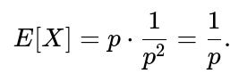
Therefore,


Hence,
Result
Thus, the expectation of a geometric random variable (defined as the count of trials up to and including the first success) is:
This holds for any 0<p≤1. If pp is 1, you will succeed immediately on the first trial, so E[X]=1, which is consistent with 1/p. If p is 0, in theory, a success never occurs and the expectation is not defined (or is infinite, depending on how you interpret the process).
Below is a brief Python snippet for simulating a geometric random variable and empirically checking its mean:
import random
import statistics

def geometric_rv(p):
    count = 0
    while True:
        count += 1
        if random.random() < p:
            return count

p = 0.3
samples = [geometric_rv(p) for _ in range(1000000)]
print("Empirical Mean:", statistics.mean(samples))
print("Theoretical Mean:", 1/p)
This simulation repeatedly generates geometric random variables and compares their empirical average to the theoretical 1/p.
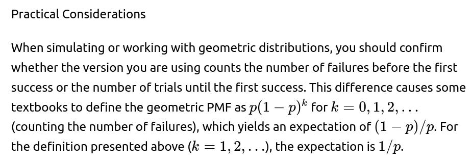
How do we handle parameterization differences?
In some contexts, the geometric distribution is parameterized by counting how many failures occur before the first success. That version would have its PMF:

In that scenario, the expected value turns into (1−p)/p. One must be sure which version is being used in any given problem or code library to avoid confusion.
What if p is extremely small or extremely large?
For very large p close to 1, the expected value E[X] is close to 1, which means you typically see a success very quickly. For very small p, the expectation grows very large. This has implications in real-world systems where “success” is rare, leading to large waiting times.
Could one derive this expectation using other approaches?
Yes. Another common way is via the notion of “memoryless” property or using a direct conditional expectation argument:
If we let X be geometric, then:

where the first term is the chance you succeed on the first trial times the immediate cost of 1 trial, and the second term accounts for failing once (thus “wasting” a trial) and then having the same distribution again because of independence. Solving for E[X] directly yields 1/p.
What are typical applications of the geometric distribution?
It is often used to model the number of attempts needed for the first success, such as the number of coin flips until the first head, the number of defective products inspected before finding the first non-defective unit, or the number of users arriving in a queue until a certain event happens. In machine learning or systems contexts, it can represent how many times you repeat a random procedure before achieving a positive outcome.
Are there practical implementation pitfalls?

Below are additional follow-up questions
Can the geometric distribution be derived using generating functions, and how does that approach compare to the series differentiation method?
One way to find the expectation of a geometric random variable is by using the probability generating function (PGF) or moment generating function (MGF). Let’s outline how the PGF approach works, since the geometric distribution is discrete.
A probability generating function for a discrete random variable X taking nonnegative integer values is defined as:

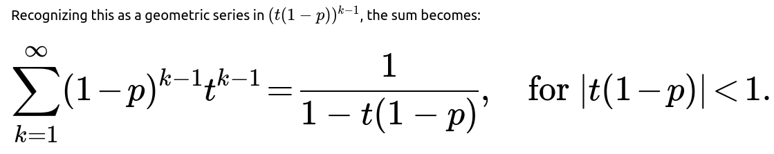

A straightforward differentiation and careful substitution of t=1 yields 1/p. This parallels the series differentiation approach but places it within the unifying framework of probability generating functions. The advantage is that if you also want higher moments or other properties, the PGF method can be extended more systematically than summation manipulations, though it’s conceptually similar.
A potential pitfall arises if you mix up the parameterization (the version that starts at k=0 for failures vs. k=1 for trials) and forget to shift indices in your generating function. This can lead to incorrect sums or an off-by-one error in the final expression.
Is there a straightforward way to compute the variance of a geometric random variable, and does it require similar summation techniques?

How do we ensure numerical stability when calculating the geometric distribution probabilities for very large values of k in software?

Approximate thresholds: For extremely small p, you might bound the probability of large k values below machine epsilon and stop computations beyond a certain cutoff.
Use built-in libraries: Many statistical libraries have specialized functions (e.g., in Python
scipy.stats) that handle edge cases internally with carefully written numerical code.If you do not address numerical stability, you may incorrectly compute distribution probabilities or partial sums, leading to inaccurate inferences or parameter estimates in real-world machine learning workflows.
How does the geometric distribution connect to the negative binomial distribution, and can that lead to additional insights about waiting times?
The negative binomial distribution generalizes the geometric distribution to the case where you are interested in the number of trials to achieve r successes (instead of just the first success). When r=1, the negative binomial distribution reduces exactly to the geometric distribution. More concretely, the negative binomial distribution’s PMF is:
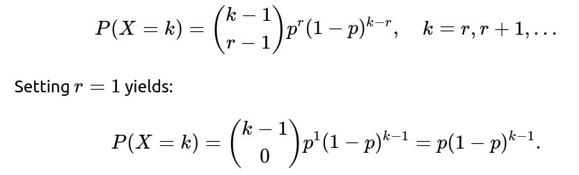
The connection is useful in modeling situations where you want to track the time or number of trials until multiple successes occur. It highlights that the geometric distribution is a special case within a larger family of discrete waiting-time distributions. One subtlety is remembering that if you want the distribution for the number of failures (as opposed to total trials) before r successes, you have a slightly altered parameterization. In practice, confusion can arise if different textbooks or libraries define the negative binomial in different ways (some start counting at zero, some at r). Always confirm which version is being used to avoid mistakes in applied settings.
Is the geometric distribution considered “heavy-tailed,” and why or why not?

However, a subtle point is that if p is extremely small, while the distribution is not heavy-tailed by formal definitions, the “practical” tail for real-world waiting times can still be quite extensive. In other words, you can still see very large outcomes with nontrivial probability if p is tiny (e.g., p=0.0001). Though it remains an exponential decay, it can be large enough to be problematic in some applications, such as queueing systems that rarely succeed.
How do you estimate the parameter p if you only observe data generated by a geometric process?

So the MLE for p is the reciprocal of the sample mean (consistent with the fact that the theoretical mean is 1/p). A subtlety is that if one observation is extremely large, it can heavily influence this estimate. That might indicate that if your distribution or data is contaminated (e.g., by outliers from a different process), your estimate of p can be severely distorted. In actual machine learning tasks, it might be wise to do robust estimation or checks for data anomalies.
What if we consider a “shifted” geometric distribution that starts counting at zero—can that alter how we compute expectations?

Thus, we have two versions of the geometric distribution:
Number of trials until first success (support = 1,2,3,…)
Number of failures before first success (support = 0,1,2,…)
When using any library function (such as in R, Python, MATLAB), you need to carefully check which version is being used. If you proceed under the wrong assumption, you’ll get an off-by-one discrepancy in your results. This can lead to confusion in real-world scenarios—say, if your domain expert states “We want the distribution of how many defective items we see before we find a non-defective,” but your software library uses the other version.
How might sampling from a geometric distribution become relevant in reinforcement learning or stochastic algorithms?
In certain algorithms where “restarts” or random durations are employed, the geometric distribution can act as a discrete analog of the exponential “memoryless” property. Examples include:
Episodic tasks with random termination: Some reinforcement learning environments might terminate with probability p on each step, leading to episode lengths following a geometric distribution.
Exploration strategies: Occasionally, one might implement an exploration schedule that tries a random action for a geometrically distributed time before returning to a default policy.
Stochastic recency weighting: The memoryless property can be exploited in weighting updates, where each update “resets” with a certain probability, ensuring you do not rely indefinitely on old states.
A pitfall is that if p is chosen poorly—either too large or too small—this can lead to episodes or exploration phases being cut too short or going on for too long, respectively. In real-world RL tasks, carefully tuning p can have a large effect on learning speed and stability.
Can a mixture of geometric distributions model more complex waiting times that do not follow a single geometric pattern?
Yes. If you suspect that your data on waiting times comes from a process with multiple “phases” or subpopulations—each with a different success probability—then a single geometric distribution might not fit well. Instead, you could consider a mixture:

Could you link the geometric distribution to reliability or “time-to-failure” models in a manufacturing context?
While continuous-time reliability models often use the exponential distribution, the discrete analog in systems that undergo discrete cycles or checks is essentially geometric. For example, if a machine is tested each morning, and each test can fail with probability p, the number of days until the first breakdown might be geometric. A real-world subtlety here is that the machine might degrade over time, invalidating the assumption of a constant probability p. If p changes with each trial (e.g., a higher chance of failure the older the machine is), the distribution no longer remains geometric. Therefore, if you see consistent upward or downward trends in the probability of “failure,” the geometric model is not correct. This can be a major pitfall in applying the geometric distribution to real maintenance problems where p is not actually constant.


