
ML Interview Q Series: Deriving Independent Poisson Distributions for Particle Counts Using Poisson Thinning.

Browse all the Probability Interview Questions here.
A radioactive source emits particles toward a Geiger counter. The number of particles that are emitted in a given time interval is Poisson-distributed with expected value λ. An emitted particle is recorded by the counter with probability p, independently of the other particles. Let the random variable X be the number of recorded particles in the given time interval and Y be the number of unrecorded particles in the time interval. What are the probability mass functions of X and Y? Are X and Y independent?
Short Compact solution
Because the total number of emitted particles N follows a Poisson distribution with mean λ, and each emitted particle is recorded with probability p (and thus not recorded with probability 1−p), one can show that:
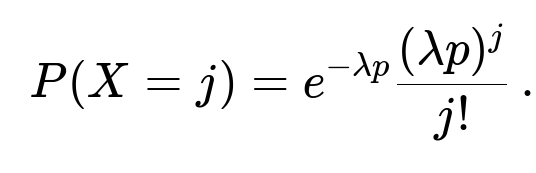
X (the number of recorded particles) is Poisson with mean λp.
Y (the number of unrecorded particles) is Poisson with mean λ(1−p).
Moreover, X and Y turn out to be independent. Concretely,


Comprehensive Explanation
Derivation from the distribution of N
Let N be the total number of particles emitted in the time interval. By assumption, N is Poisson with mean λ. Formally, the probability that N=n is:
Given N=n, each of these n particles is independently recorded with probability p. Thus, if we condition on N=n:
The number of recorded particles X follows a Binomial distribution with parameters n (the total trials) and p (the success probability).
Consequently, the number of unrecorded particles Y is n−X.
Hence, conditioned on N=n:
X has P(X=j | N=n) = (n choose j) p^j (1−p)^(n−j).
Y is then (n−j). So if we want P(X=j, Y=k), it is P(X=j, Y=k | N=j+k) times P(N=j+k), because for X=j and Y=k, the total must be j+k. This leads to:
P(X=j, Y=k) = ( (j+k) choose j ) p^j (1−p)^k e^(-λ) ( λ^(j+k) / (j+k)! ).
Using known identities for Poisson and binomial thinning, one can sum out j+k over n to find the marginal distributions. A standard (and very useful) result is that a Poisson random variable “split” into two categories (with probabilities p and 1−p) yields two independent Poisson random variables whose means are λp and λ(1−p).
Probability mass functions
Thus we obtain for all integer j≥0:

Why independence?
To show X and Y are independent, we compute P(X=j, Y=k) and compare it to P(X=j)P(Y=k). From the law of small numbers (or the thinning property of the Poisson process), the events “X=j” and “Y=k” stem from two disjoint Poisson processes, each capturing a portion of the original Poisson process of rate λ. One portion has rate λp, and the other has rate λ(1−p). The formal calculation confirms:
P(X=j, Y=k) = e^(-λp) ( (λp)^j / j! ) × e^(-λ(1-p)) ( (λ(1-p))^k / k! ) = P(X=j) P(Y=k).
Hence, X and Y are independent.
Relationship to X+Y
X+Y simply corresponds to the total number of particles N (all recorded plus all unrecorded). Indeed,
X+Y has a Poisson distribution with mean λ,
because X has mean λp, Y has mean λ(1−p), and their sum is λ. This is perfectly consistent with X+Y being the entire set of emitted particles.
Practical simulation in Python
Below is a brief snippet to simulate this scenario and empirically check distributions:
import numpy as np

def simulate_XY(lambda_val, p, num_sim=10_000_00):
    # Generate N from Poisson(lambda_val)
    N = np.random.poisson(lambda_val, size=num_sim)

    # For each N, record successes with probability p
    # This can be done via binomial or summation of Bernoulli
    X = np.array([np.random.binomial(n, p) for n in N])
    Y = N - X

    return X, Y

# Example usage
lambda_val = 5.0
p = 0.3
X, Y = simulate_XY(lambda_val, p)
# You can check empirically that X~Poisson(lambda_val*p),
# Y~Poisson(lambda_val*(1-p)), and X, Y are approximately independent.
This code first samples N from a Poisson(λ) distribution and then splits each observation into X successes with probability p and Y fails with probability 1−p. Repeated empirical analysis of X and Y would show that their empirical distributions align with Poisson(λp) and Poisson(λ(1−p)), and that sample correlations are near zero, confirming independence.
Are X and Y always independent for any distribution of N?
X and Y are not always guaranteed to be independent for any arbitrary distribution of N. The thinning property and resulting independence rely heavily on N being Poisson and each emission being recorded (or not) independently with a fixed probability p.
If, for instance, N had some other distribution or the recording process were not independent across particles, it would break the Poisson thinning property, and X, Y could be correlated. The key is that each particle’s “path” (recorded vs not recorded) is decided independently and identically with probability p, and N is itself Poisson.
What is the distribution of X given X+Y = m?
Another natural question is: if you are told that X+Y = m, what is the distribution of X? In this conditional scenario, we know there are m total emitted particles. The number of recorded ones among these m is binomially distributed with parameters m and p. Hence,
X | (X+Y = m) ~ Binomial(m, p).
This ties in perfectly with the idea that, conditional on N=m, each of the m particles has an independent chance p of being recorded.
Potential pitfalls in real-world implementations
One practical caveat is that in many real-world Geiger counter scenarios, p might not be constant if the detection hardware saturates (e.g., at high emission rates) or if environmental factors change the detection probability over time. The theoretical derivations assume a constant p for each of the N particles, and complete independence between particles. Any systematic departure from these assumptions can introduce correlations between X and Y, or cause the marginal distributions to deviate from Poisson.
Another subtlety is that λ itself might be unknown and must be estimated. In practice, one might measure the average count rates or use calibration data to estimate λ and p. In such cases, one needs to account for the uncertainty in these parameters when drawing inferences about the underlying process or when building advanced models (e.g., Bayesian approaches).
All of this underscores the elegance and power of the thinning property of Poisson processes—once you confirm that arrivals or emissions indeed follow a Poisson process, splitting those arrivals independently with probability p yields two independent Poisson processes.
Below are additional follow-up questions
If the detection probability p changes over time, how does that affect the independence of X and Y?
When p is not constant but instead varies with time or other external factors, the classic “thinning” argument for Poisson processes no longer applies in its simple form. The core assumption behind X and Y being independent Poisson random variables is that each of the N particles faces an identical and independent chance p of being recorded. If p changes over the interval—for example, p(t) is different at different times t—then the probability of being recorded is not the same for each particle. Consequently:
The total number of recorded particles over the interval will still be a random variable, call it X. However, its distribution might become more complicated than a straightforward Poisson(λp).
The distribution for Y would also change, and the sum X + Y = N could remain Poisson(λ) (if the emission process is still Poisson), but the breakdown into X vs Y would no longer follow a simple split with identical probability p for each event.
Independence generally breaks down because the variability in p over time can induce correlations. For example, if the detection probability was especially high at the beginning of the interval (leading to a higher fraction of recorded particles), that could indirectly affect how many are left unrecorded at other times, creating correlation between X and Y.
A potential pitfall is that one might incorrectly apply the thinning property by assuming p is constant and arrive at misleading estimates or confidence intervals. In real-world scenarios—especially if the detection hardware’s sensitivity or threshold changes—the assumption of a constant p can be invalid. One must either model p(t) explicitly or verify that p remains stable throughout the observation.
In practical scenarios, the Geiger counter can saturate at high emission rates. How does saturation affect the distribution or independence?
Geiger counters (and other detectors) often have a so-called “dead time” or saturating region where they cannot record new events for a short period after detecting a particle. This violates the assumption of independent recording at a constant probability p because:
Above certain count rates, the detector can miss additional incoming particles simply because it is recovering or is unable to respond immediately.
The effective detection probability depends on the current emission rate. This creates a feedback loop: high N leads to more frequent detection attempts, which can lead to more frequent detector saturation, thus lowering detection probability and injecting correlation among recorded and unrecorded events.
Consequently, X and Y would no longer be independent, nor would they each follow a pure Poisson distribution. Instead, more sophisticated models that account for dead time or saturation effects (often Markov chain-based or renewal process-based) must be used to describe the count statistics accurately.
A subtle pitfall here is that if one measures only moderate rates and sees no evidence of saturation, they might apply the standard thinning argument. But if the actual emission rate occasionally spikes above the detector’s dynamic range, the data analysis might yield systematically biased estimates for λ or p, or incorrectly conclude X and Y are independent.
If N is not Poisson, but some other distribution, do we still get the same results for X and Y?
The elegance of splitting into two independent Poisson processes relies heavily on N being a Poisson-distributed count of events. If N follows some other distribution—say, a binomial, negative binomial, or a more general compound Poisson—then X, the number recorded, will still have some distribution derived from “sampling” those N events with probability p. But it will not in general be Poisson(λp), and Y will not be Poisson(λ(1−p)):
The independence of X and Y also typically breaks down unless N has specific properties that emulate Poisson thinning (for example, if N is Poisson, or if the “thinning” process is specially designed).
Even if X and Y remain well-defined, the neat factorization of P(X=j, Y=k) = P(X=j) P(Y=k) might fail, introducing correlations.
In practice, if one sees empirical evidence that X and Y deviate from Poisson or appear correlated, it might be a sign that the underlying emission process itself is not Poisson or that p is not constant and independent across events.
Suppose we only observe X (the recorded count) but not Y. How can we estimate p and λ from the observed data?
When Y is not observed, we have partial information:
We directly see how many particles are recorded, but not how many were missed.
A single time-series of X alone, if we assume the emission is Poisson(λ) and that each event is independently recorded with probability p, can still help us estimate the product λp from the distribution of X. Specifically, we can fit a Poisson(µ) to the observed data and interpret µ as λp.
However, separating λ and p individually from µ is not possible without additional information. Essentially, if X is Poisson-distributed with mean λp, then we only know the product of λ and p from that distribution alone.
Additional data or assumptions might resolve this identification problem. For example:
If we have some external calibration data telling us the true emission rate λ (from a more accurate measuring device), then we can solve for p = (mean of X)/λ.
Alternatively, if in a portion of the experiment the detection probability is known (e.g., p=1 for a short time using a specialized setup), we can estimate λ and then revert to normal operation to estimate p.
A common pitfall is forgetting that X alone cannot disentangle λ and p without external constraints. One must be mindful of identifiability when attempting to do parameter inference.
In a real system, detection might not be strictly binary (some partial detection). How does that affect the model?
Sometimes instead of a simple binary event (recorded or not recorded), there is a more nuanced measurement process where partial signals can occur, or the amplitude of the pulse might be measured. In that case:
We might model the measurement outcome for each particle as a continuous random variable, or at least a multi-category variable indicating different “strengths” of detection.
The thinning property that leads to X and Y being Poisson random variables relies on each event being classified into one of two categories with fixed probabilities. With more than two categories or partial detection intensities, we can still generalize Poisson thinning to multi-category thinning (each category can yield a Poisson distribution under the right conditions). But the mathematics become more involved, and the independence among different categories is not guaranteed unless the classification probabilities are constant and events are independent.
A subtlety is that partial detection may allow an event to be partially recorded multiple times or recognized incorrectly in overlapping intervals, thus introducing correlation among record outcomes. Detailed models from point process theory might be needed to capture these complexities.
If an experimenter wants to build a hypothesis test to compare two different counters with different p values, what issues might arise?
When comparing two Geiger counters, each with its own probability p (say p1 for the first counter and p2 for the second counter), several issues come up:
Both counters might experience different dead times or saturations, leading to different effective p's that depend on the emission rate. This means p1 and p2 can vary in unanticipated ways if the source’s intensity changes.
If we observe X1 from counter 1 and X2 from counter 2 simultaneously on the same radioactive source, we might assume X1 ~ Poisson(λp1) and X2 ~ Poisson(λp2). But if the counters interfere with each other or if environment or geometry is different, the assumption might be violated.
Variance estimation is crucial. For Poisson(λp), the variance is also λp. For large counts, normal approximations might be used in hypothesis testing, but for smaller counts, exact or distribution-based methods are safer.
A hidden pitfall is that if we do not account for correlation that can happen through the source or the environment (like partial overlap in detection volumes), we might incorrectly conclude one detector is more efficient. Real-world measurement geometry or crosstalk effects can undermine the assumption of independence across devices, leading to flawed statistical comparisons.
How can we handle bursts or clustering in emissions where the Poisson assumption might not hold?
Radioactive emissions are often modeled as a Poisson process under the principle of random decay times. However, in some physical or experimental setups, bursts (clustering) can occur—due to chain decay processes or other phenomena—making the times of emissions not strictly memoryless:
If emissions cluster, the distribution of arrivals might have over-dispersion compared to Poisson. That is, we might observe more variance in the counts over time than a Poisson model would predict.
In such cases, using a Poisson assumption for N can systematically underestimate the probability of large bursts. The thinning argument for independent Poisson splits also fails because the arrivals are not purely Poisson to begin with.
The key pitfalls are misestimating risk levels or detection probabilities in bursty or correlated arrival scenarios. In practice, a more general point process (e.g., a Cox process or a Hawkes process) might be used, and the distribution of X and Y might show correlation or unusual tail behavior that a Poisson-based approach cannot capture.