
ML Interview Q Series: Deriving the Moment Generating Function for a Normal Distribution.

Browse all the Probability Interview Questions here.
Explain what a moment generating function (MGF) is and then derive the MGF for a normal random variable X.
Short Compact solution
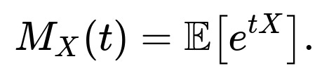
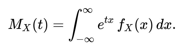
A moment generating function for a continuous random variable is defined as
For a standard normal random variable, whose probability density function is
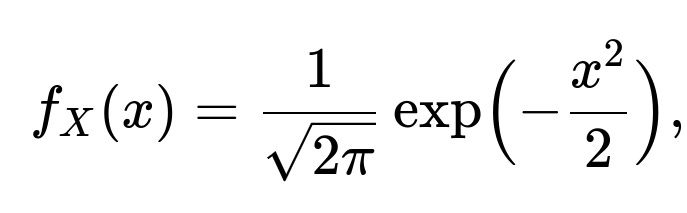
we substitute this into the integral
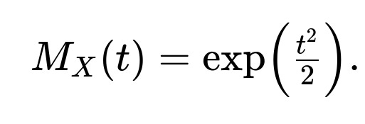
Completing the square inside the exponent and recognizing the integral is the total area under a standard normal curve, the result simplifies to
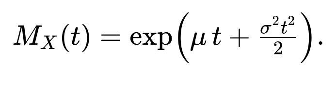
For a general normal random variable with mean ( \mu ) and variance ( \sigma^2 ), the MGF becomes
Comprehensive Explanation
The moment generating function of a random variable is a tool that summarizes all the moments (i.e., expected values of powers) of the distribution. Given a random variable ( X ), its MGF is formally defined by the expectation ( \mathbb{E}[e^{tX}] ) for those values of ( t ) for which this expectation exists. If the variable is continuous, you compute the MGF by integrating ( e^{t x} ) multiplied by the probability density function of ( X ).
One of the primary reasons the MGF is useful is that it neatly encapsulates the entire sequence of raw moments of ( X ). Specifically, if you differentiate ( M_X(t) ) with respect to ( t ) and then evaluate at ( t=0 ), you obtain the successive moments of ( X ). For instance, [ \huge \frac{d^n}{dt^n} M_X(t)\Bigl|_{t=0} = \mathbb{E}[X^n]. ]
Derivation for the Standard Normal Case
Consider ( X ) as a standard normal random variable, which has mean 0 and variance 1. Its PDF is [ \huge f_X(x) = \frac{1}{\sqrt{2\pi}} \exp\Bigl(-\frac{x^2}{2}\Bigr). ] We need to compute [ \huge \mathbb{E}[e^{tX}] = \int_{-\infty}^{\infty} e^{t x} , \frac{1}{\sqrt{2\pi}} \exp\Bigl(-\frac{x^2}{2}\Bigr), dx. ] Inside the exponent, combine ( e^{t x} ) and ( \exp\bigl(-x^2/2\bigr) ) to get [ \huge \exp\Bigl(t x - \tfrac{x^2}{2}\Bigr). ] By completing the square, you rewrite ( t x - x^2/2 ) in a form like [ \huge -\frac{1}{2}\Bigl(x^2 - 2 t x + t^2\Bigr) + \frac{t^2}{2}. ] This rearrangement highlights a Gaussian-like expression in ( x ), plus a separate constant term (\tfrac{t^2}{2}). The Gaussian-like integral then sums to 1 because it is equivalent to a normal PDF in ( x ). You are left with [ \huge \exp\Bigl(\tfrac{t^2}{2}\Bigr), ] which is the MGF for the standard normal distribution.
Extension to a General Normal Distribution
If you consider a normal random variable ( X ) with mean ( \mu ) and variance ( \sigma^2 ), you can write ( X = \mu + \sigma Z ) where ( Z ) is standard normal. Then [ \huge \mathbb{E}[e^{tX}] = \mathbb{E}\bigl[e^{t(\mu + \sigma Z)}\bigr] = e^{t\mu} ,\mathbb{E}\bigl[e^{t \sigma Z}\bigr]. ] Since ( Z ) is standard normal, we already know its MGF is ( \exp(t^2/2) ). Substituting ( \sigma t ) in place of ( t ) leads to [ \huge \exp\Bigl(\tfrac{(\sigma t)^2}{2}\Bigr) = \exp\Bigl(\tfrac{\sigma^2 t^2}{2}\Bigr). ] Multiplying by the factor ( e^{\mu t} ) outside the expectation gives [ \huge \exp\Bigl(\mu t + \tfrac{\sigma^2 t^2}{2}\Bigr). ] That is the MGF for a normal random variable with mean ( \mu ) and variance ( \sigma^2 ).
Follow-up Question 1: Why is the MGF often used in probability and statistics if the characteristic function (Fourier transform of the PDF) also exists?
The MGF and the characteristic function serve similar roles, in the sense that both uniquely characterize a distribution (under mild conditions). However, the MGF can be more convenient for some applications, particularly for computing raw moments by direct differentiation at ( t=0 ). The characteristic function, on the other hand, always exists (because ( e^{i t X} ) is a bounded function), while the MGF might not exist for certain heavy-tailed distributions if ( \mathbb{E}[e^{tX}] ) diverges. In many practical settings, when the MGF does exist in an open interval around 0, it can be easier to handle real exponentials rather than complex exponentials, making moment extraction more direct.
Follow-up Question 2: What if the MGF does not exist for some random variables?
The MGF might fail to exist if ( \mathbb{E}[e^{tX}] ) diverges for real values of ( t ). In such situations, the characteristic function (which is ( \mathbb{E}[e^{i t X}] )) remains an alternative because ( e^{i t X} ) has magnitude 1 for real ( t ). Distributions with heavier tails, such as Cauchy or certain stable distributions, can lack an MGF. In such cases, it is still possible to analyze their behavior through the characteristic function or other transforms like the Laplace transform (when it exists over specific ranges).
Follow-up Question 3: Can you use the MGF to derive all the moments of the normal distribution?
Yes, the MGF directly encodes all the integer moments of the distribution, whenever those moments exist. By taking successive derivatives of ( M_X(t) ) at ( t=0 ), you get [ \huge \mathbb{E}[X^n] = \frac{d^n}{dt^n} M_X(t)\Bigl|_{t=0}. ] For instance, for a normal variable ( X \sim \mathcal{N}(\mu,\sigma^2) ), its ( k )-th moment can be systematically computed by differentiating [ \huge \exp\Bigl(\mu t + \tfrac{\sigma^2 t^2}{2}\Bigr). ] This yields well-known formulas such as ( \mathbb{E}[X] = \mu ), ( \mathbb{E}[X^2] = \mu^2 + \sigma^2 ), and so on.
Follow-up Question 4: How would you implement a symbolic derivation of the MGF in Python?
In Python, one convenient approach is to use the sympy library for symbolic computation. Below is a brief example that outlines how you might define a random variable ( X ) with a standard normal PDF and then compute its MGF:
import sympy as sp

x = sp.Symbol('x', real=True)
t = sp.Symbol('t', real=True, positive=True)  # Typically we consider a region around 0

# Define the standard normal PDF
f_x = 1/sp.sqrt(2*sp.pi) * sp.exp(-x**2 / 2)

# Define e^(t*x)
expr = sp.exp(t*x)

# Define the MGF integral
MGF = sp.integrate(expr * f_x, (x, -sp.oo, sp.oo))

# Simplify the result
MGF_simplified = sp.simplify(MGF)
print(MGF_simplified)
The output should simplify to exp(t^2/2) which is exactly the MGF for a standard normal distribution.
Follow-up Question 5: What does it mean for the MGF to be “unique” to a distribution?
If an MGF exists for a distribution in an open interval around ( t=0 ), it uniquely identifies the distribution. This means that no two distinct distributions can share the exact same MGF in a neighborhood around ( t=0 ). This is a powerful property because it implies that if we know the MGF, we theoretically know everything about the distribution, including all its moments and how it behaves.
Follow-up Question 6: How do you interpret the exponent in the MGF for a normal distribution?
When we look at the MGF for ( X \sim \mathcal{N}(\mu, \sigma^2) ), which is [ \huge \exp\Bigl(\mu t + \tfrac{\sigma^2 t^2}{2}\Bigr), ] the terms inside the exponent reflect how the normal random variable’s “shift” (i.e., mean) and “spread” (i.e., variance) influence the growth rate of ( \mathbb{E}[e^{tX}] ). The linear term in ( t ) corresponds to the contribution from the mean ( \mu ), while the quadratic term in ( t ) corresponds to the contribution from the variance ( \sigma^2 ). As ( |t| ) grows, the quadratic term typically dominates, illustrating how larger variance makes the distribution’s exponential moment grow faster.
Follow-up Question 7: What happens if you try to compute the MGF for a random variable with very large or infinite moments?
If the distribution has extremely large or infinite moments, the integral or sum defining ( \mathbb{E}[e^{tX}] ) may fail to converge for many values of ( t ). This means the MGF might only exist in a narrower interval around 0, or might not exist at all if the tails are too heavy. In such cases, partial knowledge of the MGF in a limited domain can still provide information about the moments within that domain of convergence, but you cannot rely on the MGF outside it.
Follow-up Question 8: Could you mention a real-world context where the MGF of a normal random variable is directly applied?
In finance, the log returns of certain asset prices are often modeled as normally distributed (or at least approximately). The MGF of that normal distribution for log returns can be used in risk analysis or pricing certain instruments where moment-based approximations are relevant. Also, in queueing theory and reliability engineering, normal approximations are frequently used and the MGF helps in deriving approximate distributions of sums or means of random variables (via the Central Limit Theorem).
All these concepts together give a thorough understanding of why the MGF is a powerful tool for dealing with normal distributions, as well as with other distributions whenever the MGF exists.
Below are additional follow-up questions
How does the MGF relate to the concept of cumulants, and why might cumulants be more useful than raw moments in some cases?
Cumulants are closely connected to the MGF through the logarithm of the moment generating function. When you take the natural log of the MGF, the resulting function is called the cumulant generating function (CGF). Specifically, if
then the CGF is
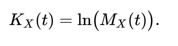
The coefficients in the Taylor expansion of (K_X(t)) around (t=0) give the cumulants of the distribution. For example, the first cumulant is the mean, the second cumulant is the variance, and so on.
One practical advantage of cumulants is that they often simplify the mathematical expressions encountered in limit theorems or expansions. For instance, cumulants can sometimes factor nicely or become additively separable when dealing with sums of independent random variables. In problems like the Edgeworth expansion (a refinement of the Central Limit Theorem), cumulants simplify the expansions more than raw moments do.
Potential Pitfall:
While moments might exist, there can be scenarios in which the MGF does not exist in an open interval around zero. In such a case, cumulants may also fail to be well-defined if we cannot take the log of the MGF in a neighborhood of zero. This usually happens for very heavy-tailed distributions.
In extremely heavy-tailed or pathological cases, higher-order cumulants might diverge even if some lower-order ones are finite. This means the CGF might be undefined beyond a certain order.
How can the MGF be used to find the distribution of the sum of two independent normal random variables?
When two random variables (X) and (Y) are independent, the MGF of their sum (X + Y) is the product of their individual MGFs. For instance, if (X) and (Y) are normal, each has an MGF of the form
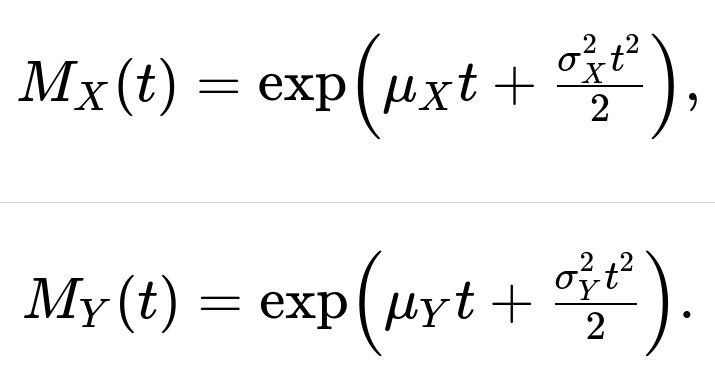
The MGF of the sum (X + Y) is:

Combine the exponents:
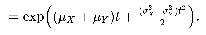
This is exactly the MGF of a normal with mean ((\mu_X + \mu_Y)) and variance ((\sigma_X^2 + \sigma_Y^2)). Hence (X + Y) is normally distributed with mean (\mu_X + \mu_Y) and variance (\sigma_X^2 + \sigma_Y^2).
Potential Pitfalls:
If (X) and (Y) were not independent, the MGF factorization (M_{X+Y}(t) = M_X(t) \cdot M_Y(t)) does not hold.
If (X) or (Y) had a distribution for which the MGF does not exist, you cannot use this approach. You might instead need the characteristic function or other methods.
In what scenarios might the MGF be misleading or provide incomplete information about a distribution?
The MGF only provides information in the region where it converges. There are distributions where the MGF exists but not on any open interval around zero. For instance, certain Lévy-stable distributions (excluding the Gaussian case) may not have an MGF that converges for (t\neq 0).
Another subtle issue is that numerical estimation of the MGF might be inaccurate for large (t). If the tail of the distribution is heavy, numerical integration or simulation-based estimates of (\mathbb{E}[e^{tX}]) can become unstable. Moreover, if you only have a truncated or approximate MGF from empirical data, you risk drawing erroneous conclusions about higher-order moments.
Potential Pitfalls:
Relying on partial or approximate MGF data to extrapolate large (t) behavior may lead to serious errors in risk modeling (e.g., Value at Risk in finance) or reliability analyses.
Misidentifying the domain of (t) for which the MGF is valid can lead to an incorrect assumption that a distribution is determined by an MGF that doesn’t actually converge.
How do you handle cases where the MGF might be valid only in a limited range around zero?
Sometimes, the MGF might converge for (t) in a finite interval ((-a, a)) around 0, but not for all real (t). In such cases, the distribution is still identified by its MGF in that interval, thanks to uniqueness results: if two distributions share the same MGF on a neighborhood of zero, they must be the same distribution.
If a question requires you to evaluate (\mathbb{E}[e^{tX}]) for (|t|\ge a), you might not be able to rely on the MGF. For large (|t|) you might explore alternative transforms like the Laplace transform for (t > 0) or other specialized techniques. Sometimes, bounding approaches or asymptotic expansions are used instead of direct MGF evaluation.
Potential Pitfalls:
Attempting to differentiate the MGF beyond the radius of convergence can lead to incorrect expressions for moments.
In numerical computations, failing to note the limited domain of convergence might result in infinite or NaN (Not a Number) outputs.
Can the MGF be used to approximate probabilities, such as (P(X > x)), using techniques like Chernoff bounds?
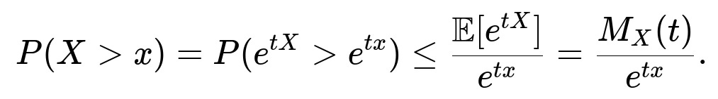
Yes. Chernoff bounds are a classic technique that leverages the MGF to bound tail probabilities. The idea is to note that for (t > 0),
Then you can minimize over (t) to get the tightest bound,
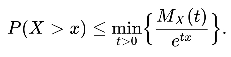
These Chernoff (or Markov) bounds can be particularly useful in large-deviation analysis and performance guarantees in fields like queueing theory or machine learning.
Potential Pitfalls:
If the MGF is infinite or doesn’t exist for some (t > 0), you can’t directly use Chernoff bounds in those regions.
Chernoff bounds, while often exponential in form, might still be loose depending on how well the MGF approximates the tail distribution.
How does symmetry affect the MGF of a distribution, and can this be exploited in some problems?
If a distribution is symmetric about zero, (X) and (-X) have the same distribution. This can impose certain properties on the MGF. For an odd moment to be zero, for example, the distribution has to be symmetric and have finite odd moments. A classic symmetric distribution is the standard normal, where the MGF is
Exploitation:
In some integrals or proofs involving the normal distribution’s MGF, symmetry simplifies the algebra.
For other symmetric distributions (e.g., certain symmetric stable laws), partial expansions of the MGF around 0 may become simpler if you know the odd-order terms vanish.
Potential Pitfalls:
Not all symmetrical distributions have an existing MGF in an interval around zero (e.g., a symmetric stable distribution with an index less than 2 might not have a well-defined MGF for (t\neq 0)).
Symmetry alone does not guarantee the existence of all moments; one must confirm moment convergence separately.
How do you empirically estimate the MGF from a sample of data, and what are common pitfalls?
You can estimate (M_X(t) = \mathbb{E}[e^{tX}]) by taking a sample (X_1, X_2, \ldots, X_n) from the distribution and computing:
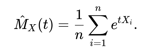
This sample mean estimator is unbiased for the true MGF at (t), provided the expectation is finite. You can do this for multiple values of (t) to get an empirical estimate of the function.
Potential Pitfalls:
If (X) has heavy tails, (e^{tX_i}) might be extremely large for some observations, causing numerical instability or skewing the average.
For large (|t|), sampling variance becomes high because (e^{tX_i}) can vary dramatically.
If the sample size is not large enough, the empirical MGF estimate can be very noisy, especially in the tail regions.
In what way can transformations of random variables (e.g., (Y = g(X))) complicate or simplify the use of MGFs?
When you perform a nonlinear transformation (Y = g(X)), the MGF of (Y) becomes ( \mathbb{E}[e^{t g(X)}]). This might be more complicated to evaluate than ( \mathbb{E}[e^{t X}]) unless (g(\cdot)) is linear. For linear transformations (Y = aX + b), it remains straightforward because
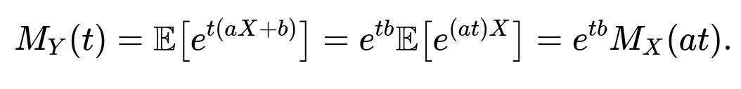
Potential Pitfalls:
If (g) is nonlinear, there may be no closed-form expression for (\mathbb{E}[e^{t g(X)}]). Approximate or numerical methods might be necessary.
Some transformations, like absolute value (|X|) or a threshold function, can cause discontinuities or kinks that make it harder to evaluate or approximate the integral defining the MGF.