
ML Interview Q Series: Deriving the PDF for Y=2X+1 via Change of Variables Transformation.

Browse all the Probability Interview Questions here.

Short Compact solution
From the provided snippet (which focuses on the slightly different variable transformation (Y = 2X - 1)), we see that:
The cumulative distribution function of (Y) can be written by expressing (X) in terms of (Y) and integrating the original (f(x)) over the appropriate interval.
Differentiating that integral with respect to (y) yields the probability density function.
It turns out (for the case (Y = 2X - 1)) that the PDF simplifies to
[
\huge g(y) ;=; \frac{2}{\pi},\sqrt{,1 - y^2,} \quad \text{for};-1 < y < 1,;\text{and }0\text{ otherwise}. ]
This is recognized as a semicircle distribution over the interval ((-1,1)).
Comprehensive Explanation
Even though the short solution snippet above specifically shows the steps for (Y = 2X - 1), the same method applies to (Y = 2X + 1). The difference is a simple shift in the range of (Y). Let us derive the PDF for the exact transformation in the question, namely (Y = 2X + 1).
Transformation Method
Given:
(X) has PDF (f(x) = \frac{8}{\pi}\sqrt{x(1 - x)}) for (0 < x < 1), and 0 otherwise.
We define a new random variable (Y = 2X + 1).
First, we note that (X) ranges from 0 to 1. Therefore:
When (x = 0), (y = 2\cdot 0 + 1 = 1).
When (x = 1), (y = 2\cdot 1 + 1 = 3).
Hence, (Y) will take values in the interval ((1, 3)).
The standard formula for the PDF of a transformed variable (Y = g(X)) where (g) is a monotonic function is: [ \huge \text{PDF of }Y ;=; f_X\bigl(g^{-1}(y)\bigr) ;\left|\frac{d}{dy}\bigl(g^{-1}(y)\bigr)\right|. ]
In our case, (g(x) = 2x + 1), so (x = (y - 1)/2). Hence (\frac{dx}{dy} = \tfrac{1}{2}).
Therefore, the PDF of (Y), which we can call (g_Y(y)), becomes:

for (1 < y < 3), and (g_Y(y) = 0) otherwise.
Plugging in the Known (f_X)
Recall that (f_X(x) = \tfrac{8}{\pi}\sqrt{x,(1 - x)}) for (0 < x < 1). Substituting (x = \frac{y - 1}{2}) inside this expression:
(x = (y - 1)/2)
(1 - x = 1 - (y - 1)/2 = \frac{2 - (y - 1)}{2} = \frac{3 - y}{2})
Thus: [ \huge f_X\Bigl(\tfrac{y - 1}{2}\Bigr) ;=; \frac{8}{\pi} ,\sqrt{,\frac{y - 1}{2};\Bigl(\frac{3 - y}{2}\Bigr)}. ] We must then multiply by (\tfrac{1}{2}) from the derivative (\tfrac{dx}{dy}).
Hence:
[
\huge g_Y(y) ;=; \frac{8}{\pi} ,\sqrt{,\frac{y - 1}{2};\frac{3 - y}{2},};\times;\frac{1}{2} ;=; \frac{8}{\pi};\times;\frac{1}{2};\times;\sqrt{,\frac{(y - 1)(3 - y)}{4},}. ] Simplify step-by-step:
Factor out the 1/4 inside the square root as 1/2 outside the square root:
[
\huge = \frac{8}{\pi} \times \frac{1}{2} \times \frac{1}{2},\sqrt{(y - 1)(3 - y)} ;=; \frac{8}{\pi} \times \frac{1}{4},\sqrt{(y - 1)(3 - y)}. ]
(\tfrac{8}{4} = 2). So:
[
\huge = \frac{2}{\pi},\sqrt{(y - 1)(3 - y)}. ]
Hence the PDF of (Y) is:

for (1 < y < 3), and (g_Y(y) = 0) otherwise.
Why It Is Also a “Semicircle” Distribution
Observe that ((y - 1)(3 - y)) can be rewritten as (-(y^2 - 4y + 3)). Shifting and factoring shows it is a mirrored, translated version of (1 - y^2). Concretely, if you let (z = y - 2), then ((y - 1)(3 - y) = 1 - z^2). Thus the resulting PDF (\frac{2}{\pi}\sqrt{1 - z^2}) is the standard semicircle shape (in terms of the variable (z)), shifted so that (z = 0) corresponds to (y=2). In other words, it is exactly the same “semicircle” form, but translated to the interval ((1,3)).
Potential Follow-Up Questions
How do we verify that this PDF integrates to 1?
To verify:
We can perform the definite integral of (g_Y(y)) from 1 to 3.
Recognize the standard semicircle integral identity: [ \huge \int_{-1}^{1} \sqrt{,1 - t^2,}, dt = \frac{\pi}{2}. ] By the linear change of variable (z = y - 2), we recast our integral over ((1,3)) into an integral over ((-1,1)). The above known identity ensures the total integral is 1 once we include the prefactor (\tfrac{2}{\pi}).
What if we had (Y = aX + b) in general?
If (X) has PDF (f_X(x)) on some interval ((\alpha, \beta)), then (Y = aX + b) would be supported on ((a\alpha + b,, a\beta + b)) (assuming (a>0)). The general formula is: [ \huge g_Y(y) ;=; f_X\Bigl(\tfrac{y-b}{a}\Bigr);\times;\Bigl|\frac{1}{a}\Bigr|. ] If (a < 0), the interval flips and you account for the negative derivative.
Can we generate samples of (Y) directly?
Yes. If you can sample (X) from the given PDF, then you can generate (Y) by simply computing (2X + 1) for each sample (X). In Python:
import numpy as np

def sample_X(n_samples):
    # Use a rejection sampler or an inverse transform approach
    # for the semicircle-like distribution in [0,1].
    samples = []
    while len(samples) < n_samples:
        u = np.random.rand()  # uniform(0,1)
        v = np.random.rand()  # another uniform(0,1)
        # We know the maximum of (8/pi) * sqrt(x(1-x)) is 4/pi at x=0.5
        # so let's do a standard rejection check
        f_val = (8/np.pi)*np.sqrt(u*(1-u))
        if v <= f_val * (np.pi/4):  # scale factor to get acceptance region
            samples.append(u)
    return np.array(samples)

def sample_Y(n_samples):
    x_vals = sample_X(n_samples)
    # Now transform
    return 2*x_vals + 1

# Example usage:
y_samples = sample_Y(100000)
print(y_samples.mean(), y_samples.std())
You would see that the (y)-samples lie between 1 and 3 and roughly follow the semicircle shape once plotted.
Are there practical scenarios where this distribution arises?
Semicircle-like distributions often appear in certain random matrix theory contexts (the Wigner semicircle law), though the exact parameters can differ. In more elementary problems, it can arise from particular Beta distributions (in fact, (X) given here is a form of Beta distribution) scaled and shifted.
What if the transformation was (Y = 2 \sqrt{X}) instead of (Y = 2X + 1)?
That would require a different approach. Specifically, you must carefully solve for (X) in terms of (Y), compute the Jacobian of the transformation, and again restrict to the domain where (X) is valid. In that case (X = (Y/2)^2), and you would have to evaluate (f_X((Y/2)^2)) multiplied by (\bigl|d/dy (Y/2)^2\bigr|). The main principle remains the same.
These kinds of transformations are tested frequently in interviews to ensure that you understand how to handle PDFs and one-dimensional variable transformations rigorously.
Below are additional follow-up questions
If (X) had a discrete distribution, can we still use the same approach to find the distribution of (Y)?
Yes, but you would have to adjust your method. For a discrete random variable (X) taking values (x_i) with probabilities (p_i), and a deterministic transformation (Y = g(X)), the probability mass function (PMF) of (Y) is obtained by summing over all (x_i) that map to a particular value (y_j). In other words, if (y_j = g(x_i)), then the PMF of (Y) at (y_j) is the sum of the probabilities of those (x_i) whose transformation equals (y_j). Formally, for each (y_j),
( \text{PMF of }Y,(y_j) = \sum_{i: g(x_i) = y_j} p_i.)
Pitfall to watch out for:
If (g) is not injective (i.e., different (x_i) values can map to the same (y_j)), you must carefully sum all relevant discrete probabilities.
Make sure that any values of (y) that are never attained by the transformation are assigned zero probability.
Hence, while the continuous approach of using a PDF and a Jacobian does not directly apply to discrete distributions, you still use the idea of “track how original values in (X) map to the new space in (Y).”
If the transformation (Y = g(X)) is non-monotonic, is the approach the same?
When the function (g) is non-monotonic, the basic formula involving the single Jacobian (\bigl|,dx/dy\bigr|) must be split into the sum of contributions from all segments where (x = g^{-1}(y)). Specifically, for a non-monotonic function that might have multiple distinct branches yielding the same (y), you need to:
Solve (y = g(x)) for all possible (x) in the support.
For each valid root (x_k(y)), compute (\bigl|\frac{dx_k}{dy}\bigr|).
Sum up these contributions to get the overall PDF of (Y).
Formally:
Pitfalls:
You might overlook some roots if (g) is piecewise or if certain branches lie outside the support of (X).
Some roots could coincide at boundary points, making it tricky to handle discontinuities or cusp points. You must carefully check endpoints.
Could we use alternative methods like moment generating functions (MGFs) to identify the distribution of (Y)?
Yes. In some cases, deriving the distribution of (Y) can be approached by working with its moment generating function (M_Y(t)) instead of directly dealing with PDFs. Recall that the MGF of a random variable (X) is:

For the transformed variable (Y = aX + b), we have: [ \huge M_Y(t) = E\bigl[e^{t(aX + b)}\bigr] = e^{tb},E\bigl[e^{t a X}\bigr] = e^{tb},M_X(a t). ]
If you can identify (M_X(t)) in closed form, you can then write down (M_Y(t)) explicitly. From (M_Y(t)), it may be possible to recognize a known distribution family (e.g., a shifted and scaled version of a known distribution). However:
This method only straightforwardly works if you can invert the MGF to retrieve the PDF (or if it matches a known pattern).
Not all distributions have easily expressible MGFs (some might use characteristic functions instead, especially if the MGF doesn’t exist in a neighborhood of 0).
Thus, while MGFs can provide insight and sometimes a direct recognition of the distribution’s form, it still requires you either to know a standard template or to manage the inversion carefully.
If the PDF (f_X(x)) has unknown parameters we need to estimate, how does that affect the PDF of (Y)?
If the original distribution (f_X(x)) has unknown parameters (for example, a Beta distribution with parameters (\alpha) and (\beta) that are not known), you would typically estimate (\alpha) and (\beta) from data using methods like maximum likelihood estimation or Bayesian inference. Once you have estimates (\hat{\alpha}, \hat{\beta}), you can plug these into the expression for (f_X(x)) to get (\hat{f}_X(x)). Then the PDF of (Y), (\hat{g}_Y(y)), follows in the same way:
[ \huge \hat{g}_Y(y) = \hat{f}_X\bigl((y-b)/a\bigr);\times;\bigl|\tfrac{1}{a}\bigr| ] (for a linear transformation (Y = aX + b)).
Potential pitfalls:
Parameter uncertainty in (f_X(x)) translates into uncertainty about the distribution of (Y). In a rigorous analysis, you might propagate that uncertainty (e.g., use a Bayesian posterior for (\alpha, \beta)).
Misestimation of parameters can lead to an incorrect shape for the PDF of (Y).
In essence, once your parameters are estimated, the “plug-in” approach is typically straightforward, but interpretational caution is needed regarding the confidence in those parameter estimates.
Could we apply this approach of transformation to a multivariate context (e.g., vector-valued (X) to some transformation (Y))?
Yes, but the procedure is more involved. For a multivariate random vector (X \in \mathbb{R}^n) with a joint PDF (f_X(\mathbf{x})), and a transformation (\mathbf{Y} = g(\mathbf{X})), one typically uses the change-of-variables formula from multivariable calculus. If (g) is a bijection and is differentiable, the joint PDF (f_Y(\mathbf{y})) is given by:
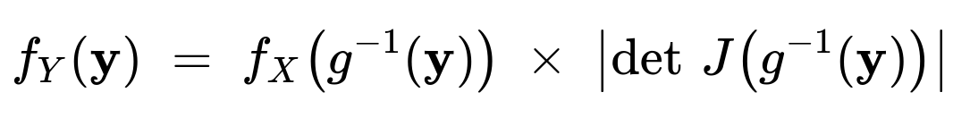
where (\det J) is the determinant of the Jacobian matrix of the inverse transformation.
Details to watch out for:
In higher dimensions, the Jacobian is a matrix (the partial derivatives of the transformation). You must carefully compute its determinant.
If (g) is not globally invertible, or if it has multiple branches, the situation is analogous to the non-monotonic 1D case—except more complicated to handle in multiple dimensions.
Domain boundaries become more nuanced: you must carefully track which region of (\mathbf{y})-space comes from which region of (\mathbf{x})-space.
In practice, how might floating-point precision issues arise when computing this PDF for (Y)?
Floating-point issues typically emerge when dealing with:
Values of (x) near the boundaries of the support where the PDF might go to 0 or approach large values. If (x) is extremely close to 0 or 1, then (\sqrt{x(1-x)}) might cause underflow or floating-point inexactness.
Repeated transformations: applying many transformations in a pipeline can accumulate numerical error.
Very small or very large numerical values in the PDF. For instance, if the PDF has a steep peak, direct computations might overflow.
Mitigation strategies:
Work in log-space when dealing with products or exponentials: store (\log(f_X(x))) instead of (f_X(x)).
Use robust numeric libraries that manage underflow/overflow more gracefully (e.g., special functions from
scipy.specialin Python).Apply bounds checking so that extremely small probabilities are treated in a controlled manner (like capping them at a small threshold to avoid zero).
If we only know the distribution function (CDF) of (X) rather than the PDF, can we still derive the PDF of (Y)?
It depends on the transformation and on whether the PDF of (X) exists. If you have the cumulative distribution function (F_X(x)) for (X), you can often find (F_Y(y)) for (Y) via:
[
\huge F_Y(y) = P(Y \le y) = P\bigl(g(X) \le y\bigr), ]
and then:
Solve (g(X) \le y) in terms of (X), and plug that into (F_X(x)) appropriately.
Differentiate (F_Y(y)) to get (g_Y(y)) if it is differentiable almost everywhere.
Even if you do not have a closed-form PDF for (X), you could numerically differentiate (F_Y(y)) to approximate the PDF of (Y). But care is needed if (F_X) is only partially known or if (g) is not monotonic. In such situations, you might have to piece together intervals of (X) that satisfy the inequality (g(X) \le y).
Main pitfalls:
Non-differentiable points in (F_X) or complicated transformations might make it hard to get a clean closed-form expression.
The derivative of the CDF might not exist if (X) has discrete components (leading to jumps rather than a smooth PDF).
Nevertheless, conceptually, the approach of “find the CDF of (Y) first, then differentiate” remains valid.