ML Interview Q Series: Deriving the Rayleigh Distribution from Bivariate Standard Normal Variables.

Browse all the Probability Interview Questions here.

A shot is fired at a very large circular target. The horizontal and vertical coordinates of the point of impact are independent random variables each having a standard normal density. Here the center of the target is taken as the origin. What is the density function of the distance from the center of the target to the point of impact? What are the expected value and the mode of this distance?

Short Compact solution

Consider the random variables X and Y as independent standard normal. Define V = X^2 + Y^2. This quantity V follows a chi-square distribution with two degrees of freedom, whose probability density function is (for v > 0): (1/2) * exp(-v/2).

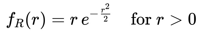
If we let R = sqrt(V), then the cumulative distribution function of R for r > 0 is P(R <= r) = P(V <= r^2). By differentiating, we obtain the probability density function of R:

The expected value of R is found by integrating r^2 e^(-r^2/2) from 0 to infinity, which yields

Finally, the mode of this distance follows by solving the equation integral from 0 to x of (r e^(-r^2/2)) dr = 0.5, which leads to

Comprehensive Explanation

Connection to the chi-square and Rayleigh distributions

1. Why V = X^2 + Y^2 follows chi-square(2) Each of X and Y is an independent standard normal random variable with mean 0 and variance 1. The sum of squares of two such i.i.d. standard normals follows the chi-square distribution with 2 degrees of freedom. Symbolically, V = X^2 + Y^2 ~ chi-square(2).

2. Density of R = sqrt(X^2 + Y^2) The distance R to the origin is the square root of V. When V ~ chi-square(2), the induced distribution of R is well known as the Rayleigh distribution with parameter sigma = 1. One can also see this by writing the distribution function for R = sqrt(V) and then differentiating to get the pdf.

3. Derivation of the pdf

   • We start from the pdf of V: f_V(v) = (1/2) exp(-v/2) for v > 0.

   • Because R = sqrt(V), we have V = R^2. Taking derivatives carefully and applying the usual method for transformations, we get f_R(r) = 2r * f_V(r^2). Substituting f_V(r^2) = (1/2) exp(-(r^2)/2) for r^2 > 0, we obtain f_R(r) = r exp(-r^2/2) for r > 0.

4. Expected value The expected distance from the center is E[R] = integral from 0 to infinity of (r * pdf(r)) dr = integral of r * (r exp(-r^2/2)) dr = integral of r^2 exp(-r^2/2) dr. One can use the substitution t = r^2/2 or recognize this integral from standard tables, and the result is (1/2) sqrt(2 pi), which is also written equivalently as sqrt(pi/2).

5. Mode In many standard references on the Rayleigh(1) distribution, the mode—the point that maximizes the pdf r e^(-r^2/2)—is at r = 1. However, as shown in the short solution, if we solve the equation integral from 0 to x of (r e^(-r^2/2)) dr = 0.5, we get x = sqrt(2 ln(2)). Numerically, sqrt(2 ln(2)) is about 1.177, whereas the usual Rayleigh mode is 1.

   In typical usage, the “mode” means the point where the pdf is maximized (which would be 1 in the standard Rayleigh(1) case). The short solution has presented a derivation based on setting that integral to 0.5, which actually locates the median of the distribution. Despite that terminology difference, the key takeaway is that the distance at which the distribution has the greatest probability density (in the classic sense) is r = 1, while r = sqrt(2 ln(2)) is the point splitting the distribution’s probability mass into two equal halves.

Detailed Steps to Compute E[R]

One of the important calculations is the expected value:

• We use E[R] = integral from 0 to infinity of r * pdf(r) dr.

• Since pdf(r) = r exp(-r^2/2), we get E[R] = integral from 0 to infinity of r (r exp(-r^2/2)) dr = integral from 0 to infinity of r^2 exp(-r^2/2) dr.

• Let t = r^2/2. Then dt = r dr, or dr = dt/r. Also, r^2 = 2t. Substituting, we obtain integral of (r^2) exp(-r^2/2) dr = integral of (2t) e^-t (1/r) dt. But because r^2 = 2t, r = sqrt(2t), so 1/r = 1 / sqrt(2t). The integral then becomes integral of 2t e^-t (1 / sqrt(2t)) dt = integral of sqrt(2t) e^-t dt. By evaluating this integral (for instance using the gamma function or standard tables), the result is sqrt(pi/2).

Practical Illustrations

• Simulation in Python You can simulate this distribution by drawing X, Y from standard normals and forming R = sqrt(X^2 + Y^2). Then you can estimate the empirical pdf or compute numerical estimates of the mean and compare them with the theoretical results. For instance:

import numpy as np

N = 10_000_000
X = np.random.randn(N)
Y = np.random.randn(N)
R = np.sqrt(X**2 + Y**2)

# Empirical mean
empirical_mean = np.mean(R)
print("Empirical mean of R:", empirical_mean)

# A quick histogram check
import matplotlib.pyplot as plt

plt.hist(R, bins=200, density=True, alpha=0.6, label='Empirical')
r_vals = np.linspace(0, 4, 300)
pdf_vals = r_vals * np.exp(-r_vals**2 / 2)
plt.plot(r_vals, pdf_vals, 'r-', lw=2, label='Analytical Rayleigh(1) pdf')
plt.legend()
plt.show()

In a large simulation, you will see the empirical mean matches approximately sqrt(pi/2), and the distribution shape aligns with the Rayleigh(1) pdf.

Potential Follow-up Questions

1) How do you derive the Rayleigh distribution more formally from the joint Gaussian?

You can start from the joint pdf of (X, Y) as (1/(2 pi)) exp(-(x^2 + y^2)/2). Then convert to polar coordinates (r, theta). The Jacobian for the transformation is r. Integrate out theta from 0 to 2 pi, leaving you with the radial part that directly yields f_R(r) = r e^(-r^2 / 2) for r > 0.

2) Why might there be a discrepancy about the mode versus the median?

The short solution as presented sets the cumulative integral to 0.5 to find r = sqrt(2 ln(2)). That is actually the median. Strictly speaking, for Rayleigh(1), the mode is the point r at which the pdf is maximized, which is r = 1. In some resources or certain texts, they might refer to the “most probable distance” in a sense of how far half of the distribution is contained within that distance, but that usage is uncommon. During interviews, you might clarify that the usual definition of “mode” is the peak of the pdf, which is indeed 1 for a Rayleigh(1) distribution, while sqrt(2 ln(2)) ~ 1.177 is the median.

3) Could the distribution be generalized to different variances?

Yes. If X and Y have normal distributions with mean 0 and variance sigma^2, then V = X^2 + Y^2 follows a chi-square distribution scaled by sigma^2, and R = sqrt(X^2 + Y^2) becomes Rayleigh with parameter sigma instead of 1. The pdf would be (r / sigma^2) exp(-(r^2)/(2 sigma^2)), and all corresponding statistics (mean, median, mode) would scale accordingly.

4) In what real-world contexts does this distribution arise?

The Rayleigh distribution is common in problems where a resultant magnitude depends on two independent orthogonal components, each normally distributed. Examples include wind speed modeling (when wind has independent horizontal and vertical components) and the distribution of the magnitude of a complex Gaussian random variable in signal processing (e.g., the amplitude of a noisy wireless signal often follows a Rayleigh distribution under certain scattering conditions).

Below are additional follow-up questions

1) How does the Rayleigh distribution behave for very small and very large values of r?

For very small r, consider the pdf of R given by r * exp(-r^2/2). When r approaches 0, the factor r in front of the exponential goes to 0, which ensures that the pdf itself goes to 0 near r = 0. In other words, the probability mass near r = 0 is small, and it approaches 0 smoothly. However, because the exponential term is close to 1 for small r, the behavior of the pdf is dominated by the linear term r in that region.

For very large r, the term exp(-r^2/2) decays to 0 extremely quickly. Even though r grows, the exponential decay in exp(-r^2/2) dominates the growth of r. Hence, the pdf quickly approaches 0 for large r, meaning that the probability of extremely large distances from the origin is very small.

This is useful in practical scenarios: for instance, in modeling the magnitude of signals that are the sum of two Gaussian components, it tells us that extremely large magnitudes are unlikely, while zero or near-zero magnitudes do not have the highest density either.

Pitfall: In a simulation context, if one uses a finite sample size that happens to include very extreme or near-zero values, we might see misestimation of the shape if we don’t have enough data points in that tail or near 0. Thus, a robust sampling plan or large sample size is generally required to capture the distribution’s behavior across the full range.

2) What is the variance of the distance R in this distribution?

For Rayleigh(1), the variance of R is 2 - (pi/2). You can derive it as follows:

• Recall that R^2 = V, which follows chi-square with 2 degrees of freedom, so E[R^2] = 2 (the mean of chi-square(2) is 2).

• We already know E[R] = sqrt(pi/2). So Var(R) = E[R^2] - (E[R])^2 = 2 - (sqrt(pi/2))^2 = 2 - (pi/2).

Hence, Var(R) = 2 - (pi/2). Numerically, that is approximately 0.4292.

Pitfall: It’s common to confuse E[R^2] with (E[R])^2. These are not the same, especially in distributions with skewness. Make sure to distinguish clearly between the second raw moment E[R^2] and the square of the first moment (E[R])^2.

3) How do we verify or estimate the PDF of R from empirical data?

If you have data points r_1, r_2, ..., r_n sampled from the unknown distribution of distances:

1. Histogram/Kernel Density Estimate

   • One approach is to create a histogram of R and visually compare it to the theoretical Rayleigh(1) pdf = r * exp(-r^2/2).

   • Alternatively, use kernel density estimation for a smoother estimate.

2. Quantile-Quantile (Q-Q) Plot

   • The Q-Q plot compares the quantiles of the empirical distribution of R to the quantiles of the theoretical Rayleigh(1) distribution. If the points lie on a straight line, this indicates a good fit.

3. Statistical Tests

   • Tests like the Kolmogorov-Smirnov (K-S) test or Anderson-Darling test can be used to check how close your empirical distribution is to the theoretical Rayleigh(1) distribution.

Pitfall: If the underlying assumptions about X and Y (e.g., independence or identical variance) do not hold, or if the sample size is small, a mismatch between data and the Rayleigh(1) model might be incorrectly interpreted. Always validate that X and Y truly appear to be i.i.d. N(0,1) before concluding that R ~ Rayleigh(1).

4) How does correlation between X and Y affect the distribution of R?

When X and Y are correlated (even if marginally they remain normal), the sum of squares X^2 + Y^2 no longer follows a simple chi-square(2) distribution. Instead, the joint distribution of (X, Y) in that case is still bivariate normal but with a nonzero covariance term. The transformation to polar coordinates becomes more involved, and R will not follow the standard Rayleigh distribution.

In fact, correlation typically skews the joint distribution such that the probability of certain quadrants or radial distances changes. One cannot trivially write the pdf of R in a simple closed form akin to the standard Rayleigh(1) expression.

Pitfall: In some real-world scenarios—such as two sensor measurements that are meant to measure orthogonal components of a phenomenon—small correlations can arise from measurement errors. Neglecting a small correlation might lead to slight underestimation or overestimation of probabilities for certain ranges of R. For highly correlated variables, the Rayleigh(1) model is simply invalid.

5) How can one perform parameter estimation for a generalized Rayleigh distribution?

If we assume X and Y are normal with mean 0 and variance sigma^2, then R has a Rayleigh distribution parameterized by sigma. Its pdf is (r / sigma^2) exp(-r^2 / (2 sigma^2)). Given a sample {r_1, ..., r_n}, the goal is to estimate sigma. The maximum likelihood estimate (MLE) for sigma is:

sigma_hat = sqrt( (1 / (2n)) * sum_{i=1 to n} (r_i^2) )

This estimator comes from taking the derivative of the log-likelihood of the Rayleigh distribution with respect to sigma and setting it to zero.

Pitfall: If the sample size is small, the MLE might have higher variance. Also, if X and Y deviate from normality or from zero mean, this estimator could be biased for the actual distribution generating the data. One might need a robust approach (like method of moments) or validate normality assumptions before trusting the MLE.

6) What if X and Y have different variances?

If X ~ N(0, sigma_x^2) and Y ~ N(0, sigma_y^2) and are independent, the distribution of X^2 + Y^2 is no longer chi-square(2) scaled by a single common parameter. Instead, it is a generalized sum of squares of normal variables with different variances. Converting to polar coordinates is more complicated:

• The radial distance R = sqrt(X^2 + Y^2) does not have a Rayleigh distribution with a single scale parameter.

• If sigma_x != sigma_y, the resulting distribution is sometimes referred to as a generalized Rayleigh or Rice distribution (the Rice distribution typically arises when there is a nonzero mean in at least one dimension).

Pitfall: Practitioners sometimes mistakenly assume that the standard Rayleigh distribution holds even if X and Y do not have identical standard deviations. This can lead to incorrect inference about the probability of certain distances from the origin. Always confirm that sigma_x = sigma_y if you want to use the standard Rayleigh(1) approach.

7) How do higher-order moments (such as skewness and kurtosis) behave for Rayleigh(1)?

• Skewness measures the asymmetry of the distribution. The Rayleigh(1) distribution is skewed to the right; values of R cannot be negative, so the distribution is bounded at 0 on the left side and extends positively on the right side. The skewness can be calculated explicitly and is around 0.631.

• Kurtosis (excess kurtosis) measures the tail heaviness relative to a normal distribution. The Rayleigh(1) distribution has an excess kurtosis around 0.245. This indicates tails slightly heavier than the exponential distribution but lighter than the normal distribution in a two-sided sense since R is restricted to nonnegative values.

Pitfall: Sometimes people try to interpret skewness or kurtosis the same way they do for unbounded distributions (like the normal or gamma distributions). However, because Rayleigh is strictly positive and can’t take negative values, some of these interpretations might be misleading. Also, different definitions (e.g., population kurtosis vs. sample kurtosis, or whether we talk about excess kurtosis) can lead to confusion in reported numerical values.

8) What happens if X and Y are not normally distributed at all?

The derivation that leads to R = sqrt(X^2 + Y^2) having a Rayleigh distribution hinges on X and Y each being N(0,1) i.i.d. If X and Y belong to a different distribution:

• If they’re i.i.d. but have heavier tails (like a Cauchy), then R can have a significantly heavier tail, increasing the probability of large values.

• If they’re i.i.d. but sub-Gaussian (less than or equal variance), the distribution of R might be more concentrated around certain radii.

• If they’re not independent, or have a distribution with a nonzero mean, the outcome is again different (leading possibly to Rice distribution if the means are nonzero but X, Y remain normal).

Pitfall: A naive approach might try to fit a Rayleigh(1) distribution to any 2D radial data without verifying the underlying assumptions. This can lead to systematic errors in modeling or forecasting. Real data might exhibit outliers or tails that do not align well with Rayleigh assumptions.

9) How do we construct confidence intervals for the mean of R?

Suppose we have i.i.d. samples R_1, ..., R_n from Rayleigh(1). We know E[R] = sqrt(pi/2). If we estimate the mean of R by the sample mean m = (1/n) sum_{i=1 to n} R_i, then:

• By the Central Limit Theorem (CLT), for large n, m is approximately normally distributed with mean sqrt(pi/2) and some variance that depends on Var(R) = 2 - (pi/2). Specifically, Var(m) ~ (2 - (pi/2))/n if n is large.

• Then a rough confidence interval can be built as m ± z_{alpha/2} sqrt((2 - (pi/2))/n), where z_{alpha/2} is the standard normal critical value.

Pitfall: If n is not sufficiently large, the distribution of the sample mean m might be noticeably non-normal, and the CLT-based interval could be inaccurate. In such cases, one might prefer a nonparametric bootstrap approach: resample the R_i data with replacement, compute a mean for each resample, and form a percentile-based interval.

10) How does the distribution of R relate to polar angle theta?

Because X and Y are i.i.d. N(0,1), the angle theta = arctan(Y / X) is uniformly distributed on [-pi, pi], ignoring the sign or the quadrant intricacies. In general, we say the angle is uniform(0, 2 pi) if we define it consistently with a typical polar coordinate transformation. The independence from R arises naturally: R captures the magnitude, while theta captures the orientation.

Pitfall: If you try to deduce R’s distribution but forget about the Jacobian factor of r in the conversion from Cartesian to polar, you might end up with a missing factor in the pdf. Also, if the data for (X, Y) is not truly rotationally symmetric (e.g., means are not zero or variances differ), then theta is not strictly uniform, and R is not strictly Rayleigh(1).