
ML Interview Q Series: Describe Mean-Shift clustering, its strengths and weaknesses, similarity-based clustering with Jaccard Index, and Self-Organizing Maps.


📚 Browse the full ML Interview series here.
Comprehensive Explanation
Mean-Shift Clustering
Mean-Shift clustering is a technique that locates clusters by iteratively shifting data points toward regions of higher density. It does so by treating the data as a probability density function and attempting to find the modes (peaks) in this density. This method starts with an initial estimate for each cluster center, then updates it according to the local mean of nearby data points, eventually converging to cluster centers.
A common way to express the update step in Mean-Shift is through a kernel function K. The key formula for computing the new center is shown below.

Here:
x is the current estimate of the cluster center.
x_i refers to the data points in the neighborhood S of x (i.e., points within the current bandwidth or window).
K(...) is a kernel function (often Gaussian, but can be others).
m(x) is the updated (shifted) estimate of the center.
Essentially, the center is shifted to a weighted average of the points around the current location, with the weights given by the kernel function K. The bandwidth (or window size) controls how large or small the neighborhood is for each shift.
Pros and Cons of Mean-Shift
Pros:
It does not require specifying the number of clusters in advance. Clusters emerge naturally based on density.
Flexible: can adapt to clusters of various shapes and sizes because it tracks local density peaks.
Converges toward modes of density, making it effective in scenarios where clusters are arbitrarily shaped and not just spherical.
Cons:
The choice of bandwidth (sometimes called the kernel width) is critical. An improperly chosen bandwidth can merge distinct clusters or split a single cluster into multiple ones.
The algorithm can be computationally expensive, especially on large datasets, because each iteration involves searching for neighbors within the bandwidth.
Results can become sensitive to outliers or sparse data distributions if the bandwidth is not chosen carefully.
Similarity-Based Clustering
Similarity-based clustering refers to a family of methods that group items based on a measure of pairwise similarity rather than explicitly modeling distance in a continuous space. The idea is to define a similarity function that compares how “close” two elements are in terms of shared features, co-occurrences, or other domain-specific factors.
This approach is especially common in text clustering (where similarity may be measured using text overlap, TF-IDF cosine similarity, or word embeddings) and in clustering sets or categorical data (where the Jaccard Index is a typical measure).
The Jaccard Index
When we deal with sets, the Jaccard Index is often used to quantify similarity. It is defined as the size of the intersection of two sets divided by the size of their union.
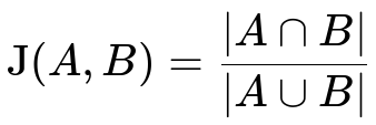
Where:
A and B are sets (e.g., sets of items, tokens, or features).
|A ∩ B| is the number of elements that appear in both A and B.
|A ∪ B| is the number of elements that appear in either A or B (or both).
A Jaccard Index of 1 means the two sets are identical, while 0 means they share no elements. This is frequently used in clustering tasks involving set-based or categorical attributes.
Self-Organizing Maps (SOMs)
Self-Organizing Maps (SOMs) are a type of neural network introduced by Teuvo Kohonen, primarily used for dimensionality reduction and clustering. They work by mapping high-dimensional data onto a lower-dimensional (often 2D) grid of neurons, preserving topological relationships in the process.
Key aspects of SOM:
Each neuron on the map has a weight vector of the same dimension as the input space.
In training, an input is presented to the map, and the neuron whose weight vector is closest to that input (in terms of a distance metric such as Euclidean distance) is deemed the Best Matching Unit (BMU).
Weights of the BMU and its neighbors on the grid are updated to become more similar to the input. This creates a “topology preserving” property: nearby neurons on the map respond similarly to similar inputs.
Over time, the map forms clusters in a way that similar data points are mapped to nearby neurons.
SOMs are especially valuable when you need a 2D view of high-dimensional data to gain insight into any natural clusters or patterns. They can also be used for tasks such as visualization or anomaly detection.
Implementation Example for Mean-Shift in Python
Below is a brief example using scikit-learn, which has a built-in MeanShift class:
from sklearn.cluster import MeanShift
import numpy as np

# Sample 2D data
data = np.array([
    [1, 2], [2, 3], [2, 2],
    [8, 8], [8, 9], [9, 8],
    [50, 50], [52, 52], [51, 50]
])

mean_shift = MeanShift(bandwidth=2)  # you can specify bandwidth
mean_shift.fit(data)

labels = mean_shift.labels_
cluster_centers = mean_shift.cluster_centers_

print("Cluster labels:", labels)
print("Cluster centers:", cluster_centers)
In real-world scenarios, you will tune the bandwidth parameter or leave it for scikit-learn’s estimate (although auto-estimation can be imprecise for some datasets).
Follow-up Questions
How do you choose the bandwidth in Mean-Shift, and what happens if it is chosen incorrectly?
The bandwidth in Mean-Shift defines the radius (or smoothing window) around each point when estimating the density. A bandwidth that is too large can merge distinct clusters into one big group because everything falls within the large window. A bandwidth that is too small might split a natural cluster into multiple sub-clusters or cause noisy assignments.
In practice, bandwidth can be chosen by heuristics such as the “rule of thumb” for kernel density estimation, cross-validation, or domain expertise. However, an optimal bandwidth is often problem-specific. If the dimensionality is high, more advanced strategies or domain knowledge are needed, as typical density estimation can suffer from the curse of dimensionality.
Why might Mean-Shift be slower compared to k-Means for large datasets?
Mean-Shift repeatedly computes density estimates and requires searching for neighbors within a given bandwidth. For each iteration, every data point potentially examines other points in its vicinity. If you have a large dataset, this neighbor search for each iteration is more computationally expensive than k-Means, which only requires assigning points to the nearest centroid and then updating each centroid.
Additionally, k-Means typically converges quickly, but Mean-Shift’s convergence depends on the density surface and can take more iterations if the bandwidth is not well tuned.
How is similarity-based clustering useful for non-numerical data?
Some data is not naturally represented in Euclidean space. For example, you might have documents, sets of categorical attributes, or graphs. In these cases, a distance measure (like Euclidean distance) can be less meaningful, but a similarity measure (such as Jaccard, cosine similarity, or graph-based similarity) can capture how alike two elements are.
This opens the door to clustering methods based on the similarity matrix (e.g., Spectral Clustering with a custom kernel, or hierarchical clustering using a specific linkage rule).
Can the Jaccard Index handle partially overlapping sets effectively?
Yes. The Jaccard Index scales with the proportion of overlapping elements. If two sets share many elements, the intersection size is high relative to the union, giving a higher Jaccard score. On the other hand, sets that overlap only slightly will result in a smaller ratio.
However, one potential issue is that if sets are very large but share relatively few common elements, the intersection may seem negligible, leading to a low Jaccard score. This result can be interpreted correctly, but it also highlights that Jaccard Index alone does not measure the absolute size difference of the sets—only the ratio of intersection to union.
How do Self-Organizing Maps differ from other neural networks like autoencoders for dimensionality reduction?
While autoencoders learn a low-dimensional latent space through an encoder-decoder framework, Self-Organizing Maps explicitly impose a 2D (or sometimes 1D or higher) grid structure to preserve topological relationships among neurons. The learning process in SOM involves competitive learning: the neuron that most closely matches the input is updated, along with its neighbors, to better match that input. By contrast, autoencoders rely on backpropagation to minimize the reconstruction error.
SOM’s discrete grid can provide a direct visual map, making it easier to interpret clusters. Autoencoders often offer more powerful compression and reconstructive abilities but are less interpretable in a simple 2D grid sense.
In what scenarios are Self-Organizing Maps a good choice?
SOMs are beneficial when:
The data has many dimensions, and you need a topological 2D or 3D representation to visualize or interpret clusters.
You desire a neural network approach with unsupervised competitive learning.
You want an interpretable, map-like structure where neighboring neurons respond similarly.
However, if your primary goal is accurate dimensionality reduction or if you have extremely large datasets, more modern techniques (like t-SNE or UMAP or autoencoders) might be more flexible or scalable. SOMs can still excel in specialized tasks where interpretability and topology preservation are critical (e.g., certain biological data analyses or smaller tasks in data mining).