
ML Interview Q Series: Describe the Isolation Forest algorithm, its benefits for outlier detection, and its anomaly identification process.


Comprehensive Explanation
Isolation Forest is an algorithm specifically designed for anomaly or outlier detection. It leverages the idea that anomalous observations are easier to isolate from the rest of the data, compared to normal points. If a point can be quickly separated from the dataset, it is likely to be an outlier. By building multiple random trees, Isolation Forest estimates how easy it is to isolate each data point. Points that have a shorter path to isolation are considered to be more anomalous.
Key Intuition Behind Isolation Forest
Unlike traditional distance-based or density-based anomaly detection methods, Isolation Forest assumes that anomalies:
Occur infrequently in the data.
Are structurally easier to isolate.
Hence, if a few random splits can isolate a point, it suggests that the point is unusual or anomalous. Conversely, a normal point typically requires more splits before it gets completely isolated.
Building the Isolation Forest
An Isolation Forest model is built by constructing multiple, shallow decision trees (referred to as isolation trees):
Each tree is grown by repeatedly randomizing both the feature selection and the split value for that chosen feature.
The process continues until a stopping criterion is met (e.g., the tree reaches a certain depth or the sub-sample size becomes 1).
Once multiple trees are built, the anomaly score is computed based on the average path length across all these trees. Shorter paths imply more anomalous points.
Core Mathematical Representation for the Anomaly Score
One common way to define the anomaly score in Isolation Forest is shown by the expression below, where E[h(x)] is the average path length of a sample x across all trees, and c(n) is a normalization factor that is dependent on the size n of the sub-samples used to build each tree:
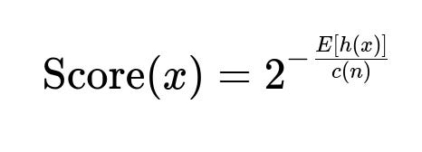
Here is an explanation of each component (in plain text for the parameters):
Score(x) in text indicates how anomalous the data point x is. Higher values denote a higher degree of “outlierness.”
E[h(x)] in text is the expected (average) path length for the point x across all the isolation trees.
c(n) in text is a constant to normalize the average path length to make scores comparable. It typically approximates the average path length of an unsuccessful search in a binary search tree of n samples, ensuring that the anomaly score remains in a meaningful range.
When Score(x) is significantly higher compared to most of the other points in the dataset, x is deemed anomalous.
Advantages of Using Isolation Forest
It focuses directly on isolating anomalies rather than modeling normal points. It can handle very large datasets efficiently because of its relatively low computational cost. It often performs well in high-dimensional settings where distance-based approaches may fail. It does not require labels; it is an unsupervised method. It is relatively straightforward to implement and interpret (shallow random splits yield short paths for anomalies).
Using Isolation Forest for Anomaly Detection
The typical steps for applying Isolation Forest to a dataset are:
Decide on the number of estimators (trees) you wish to build in the forest. This is often controlled with a parameter like
n_estimators.Sample a subset of the data points (often specified by
max_samples) to build each tree. This helps the algorithm remain efficient on large datasets.Train (fit) the Isolation Forest on your dataset. During training, the algorithm constructs the isolation trees.
Infer (predict) outlier scores for each point using the trained model. Based on a threshold (or a quantile of the distribution of anomaly scores), you label points as anomalous or normal.
A typical Python code snippet using scikit-learn:
from sklearn.ensemble import IsolationForest
import numpy as np

# Example data
X = np.array([
    [1.0, 2.3],
    [2.1, 1.9],
    [8.5, 8.8],
    [2.0, 1.5],
    [8.7, 8.2]
])

# Create and fit the model
model = IsolationForest(n_estimators=100, contamination=0.1, random_state=42)
model.fit(X)

# Compute anomaly scores (the lower, the more normal; the higher, the more anomalous)
scores = model.decision_function(X)

# Get the predicted labels: -1 for anomalies, +1 for normal
labels = model.predict(X)

print("Anomaly Scores:", scores)
print("Predicted Labels:", labels)
In this example:
n_estimatorssets the number of isolation trees.contaminationindicates the proportion of outliers we expect in our data, used to derive a threshold on the anomaly score.decision_functionyields raw anomaly scores. More negative means more anomalous.predictprovides a binary label indicating whether a point is an outlier (-1) or normal (+1).
Common Follow-up Questions
How does the choice of n_estimators and max_samples affect Isolation Forest performance?
A higher number of estimators typically yields more robust results but increases computational cost. Using an adequately sized max_samples helps generalize the notion of isolation paths without overfitting. Too small a sample might not capture the data’s general structure, whereas an excessively large sample can slow down training without significant improvement.
What are some edge cases or scenarios where Isolation Forest might struggle?
Extremely small datasets. The idea of isolation relies on random splits in a population. Very small datasets might lead to insufficient splits. Highly imbalanced data with a large number of anomalies can make it harder for the forest to discern anomalies from normal points. Non-uniform densities. If some regions have lower densities but are not actually anomalies, the algorithm might misinterpret those points as outliers. Presence of categorical variables with many levels could also pose challenges, since splits become less meaningful for categories lacking clear ordering.
Can Isolation Forest be used in an online learning scenario?
Isolation Forest as typically implemented in libraries like scikit-learn is an offline algorithm (it trains on a static dataset). For streaming or online learning environments, adjustments are needed to incrementally update isolation trees. Variants and extensions of the algorithm exist, but they may not be part of the main scikit-learn release.
How do we interpret the isolation trees themselves?
Each path in the isolation tree corresponds to a series of splits that lead to isolating a particular instance. A short average path length indicates that the instance is isolated quickly (an anomaly). By examining these splits, you can sometimes gain insights into which features caused a point to be separated from the rest of the data. This can be helpful for explainability in anomaly detection.
How do you select a suitable threshold for anomaly scores?
You can either use the contamination parameter if you have a guess about the proportion of outliers. Alternatively, you can compute anomaly scores on a validation set or a domain-specific sample of normal data. Plotting these scores or using statistical methods (e.g., percentiles) can help you choose a cutoff. Another approach is to use domain knowledge to set a maximum acceptable fraction of anomalies.
What if the data has missing values or needs preprocessing?
Isolation Forest typically operates on numerical data without missing values. You may need to handle missing data (e.g., imputation, removing incomplete entries) or encode categorical variables. Proper preprocessing ensures that random splits in isolation trees make sense and that anomalies reflect genuine irregularities, not just data encoding issues.
How do you handle feature scaling in Isolation Forest?
Isolation Forest is less sensitive to feature scaling compared to distance-based methods, because splitting is done randomly rather than based on distance metrics. However, large-scale differences among features might still affect the splits distribution. It is often advisable to scale or normalize data, especially when certain features have significantly larger numerical ranges.
In summary
Isolation Forest provides a very intuitive method for outlier detection by modeling how easily each point can be isolated. It scales well to large, high-dimensional datasets and does not require labeled data. By carefully tuning parameters like the number of estimators, sampling size, and contamination, and by applying best practices in preprocessing, you can effectively detect anomalies in many real-world scenarios.
Below are additional follow-up questions
Could Isolation Forest be integrated with other outlier detection methods, such as Local Outlier Factor or DBSCAN?
Integration of Isolation Forest with other methods typically follows an ensemble strategy in which multiple anomaly scores from different algorithms are combined. One common approach is to train separate anomaly detection models (for instance, one Isolation Forest and one DBSCAN), then for each data point, combine their anomaly scores—perhaps via simple averaging or by taking a weighted average if you have insights into which model is more reliable for specific patterns.
When combining methods:
You can achieve a more robust detection pipeline by exploiting the strengths of each algorithm. For example, Local Outlier Factor (LOF) focuses on local density comparisons, while Isolation Forest leverages isolation (partitioning) principles.
You may need to normalize scores from different models, since some methods yield inverse scales (e.g., higher scores = more normal) while others yield direct scales (e.g., higher scores = more anomalous).
A potential pitfall is the added complexity in explaining final anomalies to stakeholders, since you must clarify the logic behind each score’s contribution. Additionally, if the methods disagree strongly, you need a systematic strategy to handle such conflicts.
A real-world scenario highlighting this integration might be when you suspect that the dataset has both global and local anomalies. For instance, you can let Isolation Forest capture global outliers effectively while LOF focuses on discovering local anomalies in dense neighborhoods.
Are there domain-specific adaptations of Isolation Forest?
Yes, certain domains (e.g., cybersecurity, finance, or medical data) may require specialized adaptations or preprocessing steps before Isolation Forest can be applied effectively:
In cybersecurity intrusion detection, you might need to heavily feature-engineer network traffic data (e.g., parse packets for relevant attributes) so that random splits in feature space meaningfully reflect potential attacks.
In finance, raw transaction data often involves timestamps, geolocation, and user patterns. You might need to isolate features relevant to fraudulent behavior and possibly engineer new features (like transaction velocity or sudden location changes).
In medical data, you might integrate domain-driven transformations, such as normalizing lab tests by patient age or adjusting for measurement variability among different medical devices, so that outliers represent clinically significant deviations.
A subtlety here is that domain knowledge can significantly improve how random splits operate. If your transformations align with known risk factors or anomalies in that domain, it becomes easier for the algorithm to isolate unusual patterns.
If we only have partial anomalies labeled, can we incorporate them to get a better model?
Isolation Forest is generally unsupervised. However, if a subset of data points are labeled as confirmed anomalies (or normal), you could:
Use a semi-supervised approach: Train Isolation Forest normally, then evaluate how well it separates your labeled anomalies from the rest. If needed, you can adjust hyperparameters (e.g., contamination) or weighting to improve alignment with your labeled outliers.
Use an ensemble model: Combine Isolation Forest (unsupervised) with a supervised classifier trained on the small labeled set. The classifier might learn a boundary around known anomalies, while Isolation Forest adds a broader unsupervised perspective.
Develop a custom scoring function: One approach might be to use partial labels to refine the threshold used to decide outlier vs. inlier. Another is to incorporate labeled data in a post-processing stage to calibrate the anomaly scores.
A pitfall is that partial labels might not cover every type of anomaly in your dataset. Overfitting to a small set of known anomalies is possible, leading to missed anomalies of a different kind.
How do you interpret the decision_function output versus the raw path length in practice?
Isolation Forest typically provides:
decision_function output: In scikit-learn, a higher (less negative) value typically indicates more normal, and a lower (more negative) value indicates more anomalous. It is usually a shifted and inverted version of the raw path length to produce a more uniform range.
Average path length: This directly measures how many splits are needed to isolate a point in the trees.
When deciding how to use these:
decision_function is convenient for setting a uniform threshold across different datasets. It has built-in normalization to some degree, making it straightforward for anomaly labeling.
Raw path length can be more interpretable if you want to show exactly how quickly a point gets isolated. This can be important in debugging or explaining the anomaly rationale.
A subtlety is that the distribution of path lengths depends on how many estimators you have and your sample size. As a result, raw path lengths across different runs (with different hyperparameters) are not always directly comparable, while the decision_function attempts to maintain a more stable scale.
How do correlated features or multiple collinear features affect the performance?
Isolation Forest randomly chooses which feature to split on, so correlated features can lead to redundant splits that do not necessarily harm performance but can reduce the variety in the forest. In highly correlated datasets:
The algorithm might waste splits on essentially the same patterns in correlated features. This is less detrimental than in some distance-based methods, but can still reduce efficiency.
Because of randomization, the presence of correlations often gets “averaged out” to some extent over many trees. However, if you have extremely high correlations, you might consider dimensionality reduction (e.g., PCA) so that you remove redundant information.
In practice, moderate correlations typically do not break the method, but extremely high multicollinearity might lead to minimal gains in building additional trees.
The main pitfall is building more complex models than necessary, which can waste computational resources. But performance in terms of anomaly ranking often remains fairly robust.
If outliers cluster together, will Isolation Forest still detect them effectively?
Isolation Forest’s mechanism is to randomly isolate individual points. When outliers form a tight group (i.e., a small cluster of anomalies), there are two considerations:
The cluster might be easier to separate from normal data if that region of feature space is distinctly separate from the rest. Because random splits can isolate the whole cluster quickly, those data points might still exhibit shorter path lengths collectively.
However, if the cluster is not particularly distinct or is near the denser region of normal points, random splits may partially isolate it but not in an obviously shorter path length compared to normals.
In some rare cases, if the cluster is large enough, it might be inadvertently treated more like normal data. The algorithm’s assumption that anomalies are few and distinct could be slightly violated if you have a relatively large “outlier class” that forms its own separate cluster.
A real-world scenario might be discovering a group of fraudulent transactions from the same origin. If that origin is obviously different from the normal distribution, Isolation Forest can separate it quickly. But if it is only mildly different and the cluster is moderately large, the algorithm might not rank them as extremely anomalous.
In which circumstances might it not be suitable to use Isolation Forest?
Extremely small datasets: With too few points, random splits have limited utility, leading to unreliable isolation paths.
Large fractions of outliers: If your dataset is predominantly anomalous, the assumption that anomalies are rare is violated. The algorithm might fail to isolate them distinctly.
Highly categorical or discrete data: If your features are primarily categorical with many unique values, random splitting can become nonsensical unless carefully handled or encoded.
Situations requiring strict real-time detection with immediate updates: Since standard Isolation Forest implementations are batch-oriented, you might need specialized online variants or different algorithms.
The risk is that applying Isolation Forest in these scenarios might yield misleading anomaly scores or excessive false positives/negatives, ultimately undermining trust in the results.
Why does random splitting help, and could we do better with informed splits?
Random splitting helps the forest explore different ways of partitioning the data without biasing the algorithm. Anomalous points, which lie in sparse or “odd” regions, end up with shorter paths on average across many random trees.
Potentially, you could do better with “informed splits” if you have strong prior knowledge about which features are most relevant for anomalies. However, that might:
Introduce biases if your prior knowledge is incomplete or incorrect.
Reduce the diversity of partitions, which can decrease the algorithm’s ability to detect unexpected anomaly structures.
Moreover, implementing guided splits would complicate the algorithm, and you risk overfitting. Randomness fosters robust coverage of the feature space and usually suffices, especially when you have limited domain knowledge or the dataset is large.
Are there ways to incorporate domain knowledge or constraints into Isolation Forest?
Yes, but it often occurs outside the core algorithm’s construction phase, for example:
Feature engineering or selection. By carefully choosing or engineering features, you align the data space with known domain insights before letting random splits occur.
Post-processing or threshold adjustment. After obtaining anomaly scores, you can apply domain-specific rules. For instance, you might lower the threshold for labeling anomalies if domain experts say that certain types of misclassification are riskier.
Weighted sampling. In some advanced adaptations, you might oversample or underscore certain types of data you suspect to be more critical or more likely to contain anomalies.
A caution is to ensure that you do not disrupt the underlying assumption of random splits in a way that invalidates the algorithm. Overly constraining the splits can hinder the diversity needed for robust outlier detection.
Are there pitfalls in using Isolation Forest with extremely large datasets?
Although Isolation Forest is considered efficient, extremely large datasets can still pose challenges:
Memory constraints. Storing and processing the entire dataset for sub-sampling might exceed available memory. The
max_samplesparameter can mitigate this, but you must ensure the chosen sub-sample is representative.Time complexity. While training each tree might be fast compared to, say, a full random forest for classification, many millions of data points plus hundreds of trees can still be very time-consuming.
Over-sampling anomalies. If your random sub-sample is too small, you risk not capturing enough anomalies in each sub-sample. On the other hand, if you attempt to keep sub-samples very large, you might lose the algorithm’s speed advantage.
A real-world instance: In massive network traffic data, you might want to store and process data in streaming or mini-batch modes. If not properly configured, you risk computational bottlenecks or partial coverage of the dataset.