
ML Interview Q Series: Design a custom loss function for constrained problems like ordinal classification. Avoid misaligned objectives and instability.


📚 Browse the full ML Interview series here.
Hint: Ensuring differentiability, handling edge cases, and respecting label ordering.
Comprehensive Explanation
When dealing with unusual constraints, such as label ordering in ordinal classification, a standard loss (like categorical cross-entropy) might not fully capture the relationships between labels. Ordinal classification implies that the labels have a natural ordering (for example, “very dissatisfied” < “dissatisfied” < “neutral” < “satisfied” < “very satisfied”). A naive approach might treat them as simple discrete labels without leveraging this ordering, resulting in suboptimal training behavior. Hence, designing a custom loss function that respects ordering constraints can lead to better performance.
Unlike standard multi-class classification, ordinal classification incorporates the idea that certain classes are closer to each other than to distant classes. For instance, confusing “neutral” with “satisfied” is less severe than confusing “neutral” with “very satisfied.” Designing a custom loss involves:
Defining a suitable structure that respects the ordering.
Ensuring differentiability so the model can learn via gradient-based optimization.
Handling any edge cases (e.g., first and last categories).
Respecting Label Ordering
A popular approach is to use a cumulative link model or threshold-based model. The idea is to map the input to a single continuous output (or multiple thresholds) that determines which ordinal bucket the sample falls into. For example, if you have K ordinal labels, you can learn K-1 thresholds: t_1 < t_2 < ... < t_(K-1). The model’s output f(x) is compared against these thresholds to decide the predicted class.
One way to incorporate this into a custom loss is to ensure that these thresholds maintain a strict order. You might parameterize them in a way that enforces t_1 < t_2 < ... < t_(K-1). This can be done by learning unconstrained parameters a_1, a_2, …, a_(K-1) and then define:
t_1 = a_1 t_2 = t_1 + exp(a_2) t_3 = t_2 + exp(a_3) … t_(K-1) = t_(K-2) + exp(a_(K-1))
This construction guarantees the ordering because each new threshold is strictly larger than the previous one.
Differentiability
Differentiability is crucial. If your custom loss function involves non-differentiable components (e.g., step functions), your model’s parameters may not receive meaningful gradients. Instead of using a discrete step to enforce ordering, you can use continuous transformations (like the exponential reparameterization mentioned above). Ensuring a smooth function also typically involves using differentiable approximations (e.g., soft step functions like sigmoids or logistic functions).
Handling Edge Cases
Edge cases include small datasets, extreme imbalance in certain ordinal categories, or the scenario in which the distribution of classes is very skewed. You must ensure that your loss function:
Does not cause unstable gradients when only a few samples belong to certain categories.
Properly handles the boundary thresholds (the smallest threshold should meaningfully separate the lowest class from the next one, and similarly for the largest threshold).
Example of an Ordinal Custom Loss
A canonical ordinal regression approach (also called a cumulative link approach) might use a formulation that models the probability that a sample belongs to or is below a certain class j. If y is an ordinal label and f(x) is a learned function, you introduce thresholds theta_j for j = 1..K-1. One expression of the negative log-likelihood for the true label y could be:
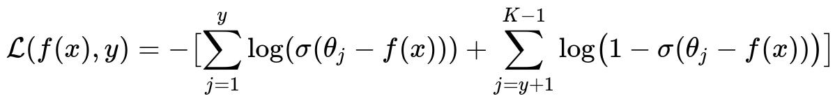
Where:
f(x) is the model’s real-valued output for a given x (the input).
theta_j for j = 1..K-1 are learnable thresholds that respect an ordering (e.g., enforced by a cumulative sum of exponential transformations).
sigma(.) is typically the logistic (sigmoid) function used to map real numbers to (0, 1).
For a sample whose true ordinal class is y, you want the probability of being in or below y to be close to 1, and the probability of being above y to be close to 0. The above negative log-likelihood penalizes deviations from these targets. Because sigmoid is smooth, everything is differentiable, allowing gradient-based training methods.
Potential Pitfalls
Overly Complex Parameterization
If you create a very complex loss function with many hyperparameters or constraints, you may struggle with optimization. Sometimes the simplest approach (like a single linear function with monotonic thresholding) is more stable.
Improper Threshold Ordering
If you do not enforce the ordering of thresholds explicitly, optimization might place them in the wrong order, violating the premise of ordinal classification. This will degrade performance and defeat the purpose of ordinal modeling.
Non-Strict Monotonicity
Even if you keep thresholds in increasing order, ensure there is a noticeable margin between them. If thresholds cluster too closely, classes become indistinguishable.
Edge Labels
For the lowest label or highest label, the model’s threshold-based logic can become degenerate if you do not handle boundary cases carefully. You must ensure that even the extreme classes provide meaningful gradient updates.
Imbalanced Data
Ordinal classes can also be heavily imbalanced. For example, you might have far more “neutral” than “extremely satisfied” samples. You might need to add class weighting or other imbalance handling to your custom loss.
Possible Implementation in Python
import torch
import torch.nn as nn
import torch.nn.functional as F

class OrdinalLoss(nn.Module):
    def __init__(self, num_classes):
        super(OrdinalLoss, self).__init__()
        self.num_classes = num_classes

        # Learnable parameters for thresholds
        # Start with random or zeros
        self.a = nn.Parameter(torch.zeros(num_classes - 1))

    def forward(self, logits, target):
        # logits: (batch_size, ) -> a single continuous output per sample
        # target: (batch_size, ) -> an integer label in [0, num_classes-1]

        # Construct thresholds that maintain ordering
        # t_1 = a1
        # t_2 = t1 + exp(a2)
        # ...
        thresholds = []
        t_current = self.a[0]
        thresholds.append(t_current)
        for i in range(1, self.num_classes - 1):
            t_current = t_current + torch.exp(self.a[i])
            thresholds.append(t_current)
        thresholds = torch.stack(thresholds)  # shape (num_classes-1,)

        # Expand logits to compare with each threshold
        # shape for logits expanded: (batch_size, num_classes-1)
        # shape for thresholds expanded similarly
        batch_size = logits.shape[0]
        thresholds_expanded = thresholds.unsqueeze(0).expand(batch_size, -1)
        logits_expanded = logits.unsqueeze(1).expand(-1, self.num_classes - 1)

        # Probability of being "below or equal" each threshold
        # We use logistic sigmoid for smoothness
        prob = torch.sigmoid(thresholds_expanded - logits_expanded)

        # For a sample whose true label is y,
        # we want prob_j~1 for j <= y, and prob_j~0 for j >= y+1
        loss = 0.0
        for i in range(batch_size):
            y = target[i]

            # product of log(prob_j) for j <= y
            # product of log(1 - prob_j) for j >= y+1
            # we sum negative log-likelihood across samples
            if y > 0:
                loss -= torch.sum(torch.log(prob[i, :y] + 1e-7))  # for numerical stability
            if y < self.num_classes - 1:
                loss -= torch.sum(torch.log(1.0 - prob[i, y:] + 1e-7))

        return loss / batch_size
In this code snippet:
We have a single logit for each instance, meaning we produce one continuous output per sample.
We learn
self.awhich reparameterizes thresholds to keep them strictly sorted.We compute probabilities for each threshold position and accumulate a negative log-likelihood accordingly.
Follow-up Questions
How do we ensure differentiability for custom constraints?
Differentiability is ensured by using continuous and differentiable functions like exponentials, sigmoids, and softplus. Instead of imposing a hard constraint (for example, threshold t2 > t1 with a step function), reparameterization with exponentials keeps everything differentiable. The key is to avoid piecewise or step-based operations that break gradient flow.
Could we do this with multiple logits instead of a single logit?
Yes. One approach is to have multiple outputs, each corresponding to the probability of being in each ordinal class. You then encode ordinal constraints by penalizing deviations in a structured way. However, a single logit plus multiple thresholds is a more direct way of reflecting the ordinal structure. If you do multiple logits, you risk losing the strict ordinal relationship unless you incorporate constraints across the logits.
What if the class distribution is highly imbalanced?
With ordinal data, imbalance is common. You can incorporate class-weighting into the loss, or employ techniques like focal loss adaptation. This might involve multiplying the negative log-likelihood terms by a weight factor that is inversely proportional to the frequency of each class, ensuring that rare classes still receive sufficient gradient.
How do I interpret threshold parameters after training?
After training, the thresholds indicate boundaries in the continuous logit space. If your model output is below t_1, the sample is in the lowest class; between t_1 and t_2, it’s in the second-lowest class, and so on. These thresholds reflect the model’s learned boundaries for different ordinal categories.
What if labels are not strictly ordinal but somewhat ordinal?
If the labels only partially follow an order, deciding whether an ordinal approach truly helps can be tricky. Purely ordinal losses might overly constrain the model. You might switch to a hybrid approach or a standard multi-class approach if the ordering is weak. Always confirm that the ordinal assumptions hold in real-world data.
Below are additional follow-up questions
How could we approach ordinal classification if the dataset is extremely large and has many distinct ordinal classes?
When the number of classes K becomes large (e.g., a rating scale from 0 to 100 or an even broader range), the threshold-based approach may still work but can become computationally and memory intensive. You have multiple thresholds (K-1), which each need to be learned and respected in a strict ordering. Training complexity can scale, and batch-based gradient updates need to accommodate many possible boundaries.
One pitfall is the potential for slow training if each sample’s loss computation has to iterate over all K-1 thresholds. You can optimize by vectorizing the computation and potentially parallelizing the thresholds. However, memory usage might still grow if you expand logits and thresholds in naive ways.
Another subtle edge case is threshold collisions or near-collisions when K-1 is large. Even a small deviation in parameters can cause thresholds to clump together, making adjacent classes hard to distinguish. Monitoring threshold spacing or applying mild regularization to spread them out can be helpful.
What if we only have partial ordering among some labels but not a strict total ordering?
In many real-world problems, certain groups of classes might follow an order, while others are incomparable. Imagine an e-commerce scenario: “small,” “medium,” and “large” are strictly ordered by size, but “custom-sized” might not fit neatly into that linear chain. In these cases, a purely ordinal strategy could be too rigid.
One approach is to build a hybrid loss function that treats part of the problem as ordinal (for the comparable labels) and part as either multi-label or multi-class for the labels that do not strictly compare. For instance, you could have separate output heads: one for the strict portion with ordinal thresholds, and another for the incomparable portion with standard cross-entropy classification.
A pitfall is forcing an order where it does not exist, which can degrade accuracy. Another subtlety is that partial orders can create disconnected label subgraphs, and simple threshold-based methods cannot handle that scenario unless carefully extended. Data scarcity in some sub-ordered sets can further complicate the training.
How do we handle real-time scenarios where the distribution of ordinal labels might shift over time?
Real-world systems often face concept drift, meaning the data distribution or label boundaries change over time. If you rely on static thresholds learned from historical data, the model might degrade in performance. In an ordinal context, even the relative spacing between classes can shift.
An incremental or online learning approach can adapt thresholds as new data arrives. For instance, you periodically update the threshold parameters with mini-batches of fresh data. Alternatively, you can keep a small buffer of recent samples to re-estimate or fine-tune the thresholds.
A common pitfall is overfitting to short-term fluctuations in the distribution if you adapt thresholds too aggressively. Conversely, if you fail to adapt enough, you might miss genuine distribution shifts. Hyperparameters controlling the frequency and scale of threshold updates must be tuned carefully.
Can we incorporate cost-sensitive considerations for different types of misclassifications in ordinal classification?
Yes. In many practical problems, misclassifying a sample by two steps (e.g., predicting “very satisfied” instead of “neutral”) might be more costly than an adjacent error. You can add cost weights that scale according to the distance between the true label and the predicted label. For example, an error margin of 2 steps might incur twice the penalty of a 1-step error.
One way to incorporate this into a threshold-based loss is to weight each individual log-likelihood contribution by a function of how far the threshold index is from the true class. Another technique is to replace uniform negative log-likelihood with a weighted version that penalizes further distance more heavily.
The challenge is choosing or estimating the cost function. If the cost matrix is not well-defined or changes across use cases, you might over-penalize certain misclassifications. There is also a risk that the model overfits to specific misclassification penalties and generalizes poorly. Hence, thorough domain research is needed to ascertain realistic misclassification costs.
What if noisy or uncertain labels exist for some samples, especially near boundary thresholds?
Ordinal data can be noisy, particularly near the boundaries between categories (e.g., when the difference between “neutral” and “dissatisfied” can be subjective). If you assume absolute correctness of the ordinal label, your threshold optimization might be misled by mislabeled or ambiguous samples.
One technique is to incorporate label uncertainty directly into the loss, for example by assigning probability distributions instead of hard labels. If a label y is ambiguous, you can create a distribution over y-1, y, and y+1. The model then minimizes an expectation of the negative log-likelihood across these plausible classes. This naturally softens the boundaries.
A pitfall is that artificially broadening distributions can degrade performance when you do have confident labels. Another subtlety is how to measure the “confidence” or “uncertainty.” Relying on heuristics or forced user input (e.g., “How confident are you in this label?”) can be challenging and might introduce further bias.
How might we adapt a threshold-based approach if we decide to break the ordinal problem down into multiple binary decisions?
An alternative perspective is to treat ordinal classification as a sequence of binary questions: “Is the label at least class i?” for i in 1..K-1. You effectively have multiple heads, each outputting a probability. For sample x with label y, all heads up to y should output 1 (true), and heads above y should output 0 (false). This is sometimes called a “one-vs.-remaining” ordinal decomposition.
While this approach naturally encodes ordering (since all heads i up to y must fire positively), it also has pitfalls. The heads might learn conflicting boundaries if not constrained to be monotonic. Additionally, if each head is an independent subnetwork, you might have a large parameter count and risk overfitting on small datasets. Another subtlety is bridging the gap between each binary output and the final single class prediction, which requires combining them consistently and ensuring no head “fires” out of order.
What if we only have coarse ordinal labels, but the underlying phenomenon is continuous?
In many real-world scenarios, ordinal labels are discrete proxies for an underlying continuous variable. For example, pain levels from 1 to 10 are discrete states in a patient’s self-report, but the true sensation is continuous. If the true distribution is continuous, forcing the model into discrete ordinal bins might lose some fidelity.
A pitfall is artificially limiting the model’s expressiveness. If you suspect continuous structure, you could treat the problem as a regression and map the continuous output to discrete bins at inference. Alternatively, you can combine the benefits of a continuous output with the interpretability of discrete class boundaries by having a single regression head and learned discretization thresholds.
The challenge is ensuring the model is not penalized too heavily for small differences that cross a single threshold boundary. In edge cases, a patient rating their pain as 4 instead of 3 might be clinically insignificant, but in ordinal classification it’s a distinct category. Properly weighting small boundary-crossing errors in a custom loss can help mitigate abrupt penalty jumps.
What steps would you take to debug a custom ordinal loss if the model’s performance is unexpectedly poor?
Debugging a custom loss function often involves systematically isolating potential issues:
Check Basic Implementation. Ensure the code that calculates the loss aligns with the mathematical intent. A small indexing error or sign error can ruin training.
Monitor Threshold Evolution. Visualize how thresholds move during training. If they do not move from initialization or collapse to a single value, you likely have gradient flow problems.
Compare to a Simpler Baseline. Try a straightforward approach such as standard multi-class cross-entropy to see if the custom approach is significantly worse. Sometimes simpler methods work better if your ordinal constraints are not strongly enforced by the data.
Use Synthetic Data. Generate synthetic ordinal data with known thresholds and see if your model can learn them. Failing on such a controlled problem often indicates implementation bugs or fundamental flaws in the loss design.
Examine Gradient Magnitudes. If gradients for thresholds or model parameters vanish or explode, you might need gradient clipping, different initialization, or reparameterizations to stabilize updates.
Look for Data-Label Mismatch. Some ordinal labels might be mislabeled or out of order (e.g., a rating of 4 in a context that logically cannot exceed 3). Such anomalies can derail threshold training.
A key pitfall is over-focusing on the raw final accuracy or mean absolute error. In an ordinal setting, you should also track whether thresholds remain in a valid order and how the model distributes predicted classes relative to the data distribution. If most predictions collapse to a single class or two, debugging threshold parameter updates becomes paramount.