ML Interview Q Series: Designing nDCG Metrics for Comparing Personalized Show Rankings

📚 Browse the full ML Interview series here.

32. How would you design a metric to compare rankings of lists of shows for a given user?

This problem was asked by Netflix.

One common challenge at Netflix is to measure how different ranking algorithms perform, specifically for each user’s preference. For instance, if you have two different ranked lists of shows for the same user, how do you compare which list better matches the user’s true preferences? This question focuses on designing or choosing a metric that can capture the difference (or similarity) between these two rankings in a meaningful way.

Below is a thorough, in-depth explanation and reasoning on how one might approach the design of such a metric, along with several potential follow-up questions and their detailed answers. Throughout, the concept of comparing ranked lists for a user’s taste is explored extensively. While describing the mathematics, the aim is to focus more on the conceptual understanding. However, a few important formulas are shown to illuminate key concepts.

A Key Idea of Ranking Metrics

One core goal is to measure, for each user, how well a predicted ranking aligns with the user’s true preference. Often, we have some notion of a ground truth ranking (or partial ranking) of items—perhaps gleaned from the user’s viewing patterns, explicit ratings, or other signals. Then, we generate a ranked list from our recommendation algorithm. We want to see how close this predicted ranking is to the ground truth.

Possible Approaches to Ranking Metrics

A widely used family of metrics includes Kendall’s Tau, Spearman’s Rank Correlation Coefficient, Discounted Cumulative Gain (DCG), Normalized DCG (nDCG), Mean Reciprocal Rank (MRR), and more. Each of these has different strengths and trade-offs. In some settings—like Netflix recommendations—it is especially helpful to consider top-weighted metrics that focus more on whether the top few positions match the user’s true top preferences.

Designing a Metric That Emphasizes Top k Items

In many recommendation systems (e.g., Netflix), the items at the top of the list are far more critical than the items at lower positions. A user is more likely to notice or interact with the first few recommended shows. Hence, a good ranking metric often focuses heavily on the correctness of the top elements. One approach is nDCG, which heavily weights the top positions by applying a decreasing discount factor as we move down the list.

How nDCG Works

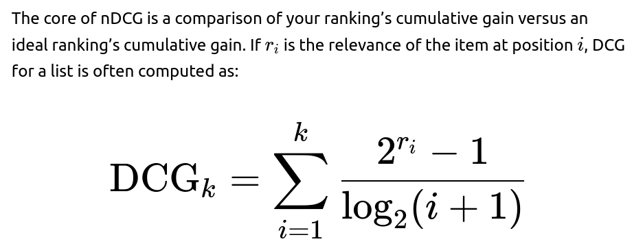
The intuition is that an item’s importance is exponentially higher if the user is truly enthusiastic about it (e.g., it could be a “top preference”). We divide by a logarithm of the rank so that getting the correct items at the top is more important than getting items correct at lower positions. Then, nDCG is formed by normalizing DCG with respect to the ideal ranking so that the best possible ranking yields nDCG = 1. This normalization helps compare across different users even if they have different preference distributions.

Why Emphasize the Top of the List?

If Netflix is recommending 10 items at a time, but the user only looks at the first few suggestions, ensuring the top part of the list aligns with the user’s preferences is crucial. nDCG is one of the best-known metrics in this regard. If one wants to focus even more sharply on the top results, variants such as nDCG@k or other top-k metrics can be used. Alternatively, metrics like Mean Reciprocal Rank (MRR) place a large emphasis on the position of the first relevant item.

Spearman’s Rank Correlation and Kendall’s Tau

Sometimes, we have not just a top k list, but a complete ordering of all items. If each user has a known (or partially known) preference ordering over a set of items, we can use correlation-based metrics such as Kendall’s Tau or Spearman’s Rank Correlation to measure how similar two orderings are. Although these are more classical rank correlation metrics, they can be relevant when:

You have full rankings or close to it (e.g., the user has provided a rating or preference for most shows). You do not particularly need to emphasize the top portion (though in many recommendation systems, you do).

where n is the total number of items.

Spearman’s Rank Correlation, on the other hand, measures how similar two rankings are by computing the Pearson correlation between their rank positions. This can be described as:

Why Not Always Use Spearman or Kendall’s Tau?

In many real-world recommendation scenarios (particularly Netflix), the user’s ground truth preference is not a total order but rather partial or uncertain. Moreover, the top of the list matters disproportionately more. Spearman’s rank correlation and Kendall’s Tau treat all positions equally—an error at position 1 is the same as an error at position 10 in these metrics. This might not align with the business or user experience priorities.

Pairwise Preference Consistency Approaches

If the data about each user consists of pairwise preferences (e.g., the user likes show A more than show B), a metric can be designed to see how many such pairwise preferences are satisfied by the predicted ranking. A simple approach: count how many user-labeled preferences are consistent with the order in the predicted ranking. You can convert that into a fraction or percentage to measure how well you respect the user’s preferences. This approach is related to the pairwise nature of Kendall’s Tau, but can be adapted to partial preference data.

Potential Hybrid Metric

In some advanced scenarios, you might combine nDCG (focusing on the top few items) with pairwise preference checks (covering partial preferences that might not be captured in explicit ratings). This ensures you measure both the correctness of your top positions and your consistency with user-labeled preferences across the entire set.

Implementation Detail with Partial Feedback

Choosing a Metric for Netflix’s Context

In Netflix’s world, the top recommended items are crucial. Hence, nDCG@k is a popular choice because it is top-weighted and normalized across users. Another dimension is personalization: some users watch a large variety of shows, others watch very few. This might lead to scenarios where naive top-k metrics can skew the results if the user’s preference distribution is particularly narrow or broad. For these reasons, Netflix has also explored Weighted nDCG or other variants that try to adapt to different user behaviors.

Real-World Pitfalls

Sometimes a user’s true preference is unknown or incompletely observed. If they only watch a small sample of recommended items, it might bias your metric. You might be measuring how well you match the user’s ephemeral mood, not their long-term interest. Another subtlety arises if you try to incorporate diversity or novelty—maybe the user’s immediate top preference is always the same genre, but Netflix wants to nudge them towards interesting new genres. In that case, the metric might need to reward variety, not just alignment with the immediate “most likely” picks.

Conclusion on the Metric Design

A metric to compare two rankings of shows for a user should reflect that user’s underlying preferences, weigh heavily the correctness of top recommendations, and ideally be robust to incomplete data. nDCG@k is a popular choice. If you need a direct measure of how often the predicted order aligns with user preferences pairwise, Kendall’s Tau or a pairwise accuracy measure can be considered. Combining different metrics or customizing them to Netflix’s unique feedback signals can give the best measure of real-world success.

32.1 How would you handle ties in user preference when designing your metric?

Sometimes the user might exhibit ties in preference. For example, they might watch multiple shows in the same session or have equally strong signals for them. This complicates ranking comparison because a standard metric like Kendall’s Tau assumes a strict ordering. If the user is indifferent between show A and show B, we can incorporate that into a pairwise metric by ignoring that pair or by designating them as “equally preferred.”

In nDCG, if we assign them the same relevance score, it does not matter which one is placed first in the ranking from the perspective of DCG. However, if we want to ensure the metric explicitly accounts for ties, we can define partial ordering acceptance in the pairwise comparisons or treat ties as a separate category where there is neither a penalty nor a reward for flipping the order of those tied items.

32.2 If some shows are newly introduced (cold-start problem), how would your metric handle them?

New shows or cold-start items may have minimal user data. The metric could assign a default relevance level for new items or omit them from the ground truth ranking until more data is gathered. Alternatively, we might treat them as “unknown” or “neutral” preference. A pairwise preference approach might simply avoid counting pairs involving items we have no information about. For nDCG-like metrics, you might set their relevance to 0 initially, or use average popularity-based relevance as a prior. Once you see user signals (watch time, rating, etc.), you update their relevance scores.

32.3 How do you evaluate the metric’s reliability across users with very different behaviors?

Users vary drastically: some watch everything from a single genre, others watch a wide variety. We often aggregate user-level metric scores (like nDCG@k) across many users to get a global measure. However, there can be distributional shifts if some users have extremely sparse data. One practical approach is to segment users based on their activity level or on how many ratings they have provided. You can then compare average metric scores across these segments. This helps reveal if your metric is stable or if it might be misleading in certain segments.

Another approach is to perform significance tests or bootstrap sampling of users to see if differences in metric scores between two ranking methods are statistically significant. In Netflix-scale data, you typically have large user populations, so you can do robust statistical comparisons.

32.4 Why might you choose nDCG over simpler metrics like precision at k?

Precision at k simply measures how many of the top k recommended items are relevant to the user. This is a coarse measure because it does not differentiate the position within the top k. For instance, placing a relevant item at rank 1 versus rank 5 is not distinguished if we are only measuring precision at 5. But in a user interface, the topmost slot might be the most visible or the most clicked. nDCG uses a logarithmic discount factor so that an item at position 1 is more influential than position 5. This captures the intuition that more relevant items should appear as high in the list as possible. Additionally, nDCG can handle multi-level relevance (not just binary relevant/irrelevant). That gives more nuance in capturing user preferences.

32.5 What if the ground truth preference itself is uncertain or changes over time?

Users’ tastes are not static, and the notion of a single ground truth ranking can be unreliable if user preferences evolve. One approach is to weight recent interactions more heavily. Another is to measure the ranking quality over time and see if the system adapts to the user’s changes. In practice, Netflix might evaluate each day’s recommended list against that user’s subsequent viewing data. If the user’s behavior changes, the ground truth can also shift. This can be captured by approaches such as time-decay weighting in the metric’s relevance scores.

32.6 How would you compute these metrics in practice at scale for millions of users?

Typically, large-scale systems like Netflix implement this in a distributed setting. You would gather relevant data (users’ watch logs, ratings, partial watch signals), compute user-level ground truth relevance vectors or partial rankings, generate the recommended lists for each user from your algorithm, and then:

Compute an incremental DCG-like score for each user’s recommended list. Aggregate or average those scores across users. Keep track of standard error or confidence intervals for these aggregate metrics.

This is done in parallel for many users in a distributed framework like Spark or through a pipeline in the Netflix data infrastructure. The final aggregated metric helps the recommendation team compare different algorithms.

32.7 Are there scenarios where your metric might fail or be misleading?

An example scenario is if the system consistently recommends the same set of popular shows for everyone. This might yield a decent nDCG if many people happen to watch those popular items. However, it might fail to personalize effectively for niche users. The aggregated metric might look good, but in practice, it means you are ignoring personalization for smaller user segments. Another scenario is if a user’s explicit rating is not aligned with their watch behavior. For example, the user might rate a show poorly but still watch it out of curiosity or background noise. The metric might get confused if the “ground truth” label and user’s actual behavior do not align.

32.8 How might you combine offline metrics with online A/B tests?

Metrics such as nDCG or pairwise preference accuracy can be computed offline using historical data. However, the real question is whether the new ranking approach improves actual user engagement, retention, or other key product metrics. Therefore, Netflix also runs online A/B tests. If a new algorithm leads to a higher offline nDCG but does not show improvements (or worsens engagement) in an online experiment, that suggests the offline metric might not fully capture the true user experience. Netflix typically uses offline ranking metrics to filter out poor approaches, then tests promising methods in online experiments to see the real user impact.

Follow-up Question 1

How might you approach designing a custom ranking metric that accounts for both user satisfaction and content diversity?

A metric that only rewards aligning with immediate user preferences might end up recommending the same genre repeatedly. However, Netflix also wants to expose users to diverse content to help them discover new shows. One approach is to design a metric that is partly based on accuracy (like nDCG) and partly on diversity. For example, you can penalize the ranking if multiple items in the top k belong to the same small sub-genre. Another approach is to measure the coverage of different categories over many recommendations. You could define a “diversity factor” that measures how many distinct genres or categories appear in the top k. Then combine that with your standard nDCG:

Compute user-based nDCG for each recommended list. Compute a diversity metric, for instance, the number of distinct genres or an entropy-based measure of category distribution. Combine them, perhaps as a weighted sum: weighted_score = α × (nDCG@k) + (1 - α) × (diversity_metric).

Choosing α might require testing to see what trade-off yields the best user experience. This approach tries to ensure that while you still recommend relevant items, you do not saturate the list with highly similar content, which can harm long-term user engagement.

Follow-up Question 2

How can you handle partial watch data when determining the ground truth relevance?

Netflix has extremely granular data: it knows how many minutes of a show a user watched, whether they finished an episode, whether they binged multiple episodes, or abandoned a show early. These signals do not translate neatly into classical “relevant vs. irrelevant” labels. A practical approach is to assign a numeric “relevance” or “engagement” score:

Maybe set a threshold for partial watch time. For instance, if the user watched at least 50% of an episode, consider it relevant. If the user completed at least one season, consider it highly relevant. If the user gave a thumbs up or a 5-star rating, assign an even higher relevance. If they quickly abandoned it, consider it less relevant or irrelevant.

Such a heuristic can be turned into a multi-level relevance scale—for instance: 0 = never clicked 1 = clicked but abandoned quickly 2 = partial watch 3 = completed a season 4 = repeated multiple seasons 5 = strongly positive rating

Then feed these multi-level labels into a DCG calculation:

Follow-up Question 3

Could you explain the intuition behind the logarithmic discount in DCG?

The essence of DCG is that items near the top of the list have a much bigger impact on the user experience than items further down. The logarithmic discount accomplishes the idea that the difference between placing an item at rank 1 vs. rank 2 is bigger than the difference between rank 9 vs. rank 10. Mathematically, this means:

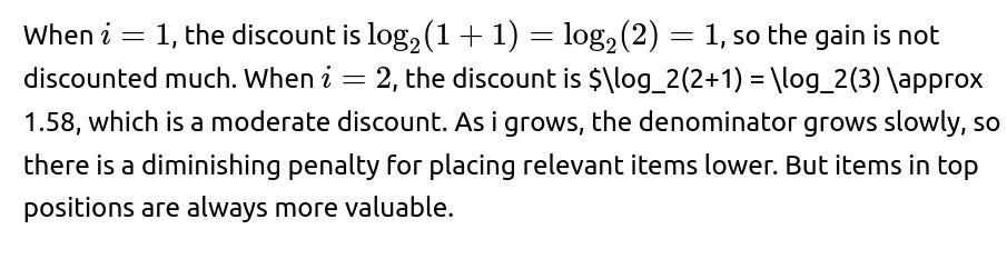
This closely aligns with how most users interact with a ranked list: they spend more attention on the top positions. Using a log discount is just one choice; you could use other discount functions (e.g., exponential discounting) if you want a steeper or gentler emphasis on top positions.

Follow-up Question 4

How could you adapt the metric if you want to measure ranking performance for a set of items that the user has never interacted with before?

This scenario arises in cold-start or novelty-focused recommendations. If the user has never interacted with these items, we lack a direct ground truth label. One approach is to measure engagement post-facto. Present the user with these new items in the recommended list, then observe the user’s subsequent behaviors. Compare the predicted rank to a realized “engagement rank” after the fact (how quickly or frequently the user watched them). Over time, you gather data that transforms “unknown” items into some level of relevance label. Another approach is to incorporate user similarity or item similarity signals, inferring that if similar users loved a show, it might be highly relevant to the current user. In practice, there is no perfect solution for brand-new items without user feedback, so you treat them with a best guess or partial label until real feedback arrives.

Follow-up Question 5

Is there a recommended approach if user preferences are context-dependent, for example, changing by time of day or who the user is with?

If the user is watching alone in the afternoon, they might prefer certain shows, but if they watch with friends or family at night, they might prefer different shows. In this context, the concept of a single universal ranking for the user might be too simplistic. One strategy is to collect contextual data (time of day, whether multiple profiles are watching, etc.) and produce context-specific relevance labels. Then you effectively have multiple ground truth preferences or partial preferences for each user—one for each context. You can compute metrics in each context separately. For instance, you can maintain an nDCG for “weekday solo watch” vs. “weekend family watch.” When you average them, you get a sense of how well your ranking does across multiple contexts. This is more nuanced and might require a deeper personalization approach that includes contextual signals.

Follow-up Question 6

How do you handle the case where the user never interacts with the top recommended items, but you are still fairly sure they are relevant?

It can happen that a user is highly likely to enjoy certain shows, but they never explicitly click them because they are always returning to Netflix to watch a particular continuing series they are already in the middle of. They might skip your top recommended shows simply because they are on a “one-track mind.” This leads to a mismatch: your metric might penalize your ranking approach because the user is not interacting with these “new” shows. But from editorial curation or external knowledge, you might still believe they are relevant. One pragmatic approach is to incorporate user surveys, or track “time to eventual watch.” If the user eventually tries the recommended show and rates it highly, that might retroactively confirm your top recommendation was good. Metrics can be smoothed over time so you are not penalized too heavily for short-term user inaction.

Follow-up Question 7

Why is normalized DCG more useful than raw DCG in comparing across different users?

Each user might have a different maximum possible DCG due to differences in how many items are relevant or how relevant they are. For instance, some users might have many high-relevance items, others might have very few. If you just look at raw DCG, the user with more relevant items in the dataset can more easily achieve a high DCG. By normalizing (i.e., dividing by the ideal DCG for that user), nDCG@k ranges from 0 to 1 for each user, where 1 means you perfectly matched the user’s best possible ordering. This allows you to aggregate fairly across users because each user’s metric is scaled relative to their own maximum possible gain.

Follow-up Question 8

What subtleties might arise if we try to measure ranking similarity among multiple candidate algorithms, not just comparing one algorithm’s ranking to the ground truth?

Sometimes you want to see how two algorithmic rankings differ from each other, ignoring the ground truth. For example, you might measure the “diversity” among algorithms that you plan to ensemble. A measure like Spearman’s Rank Correlation can tell you if two algorithms produce very similar or quite different orderings. This helps if you want an ensemble to have complementary strengths. However, if your goal is user-centric accuracy, a metric comparing each algorithm’s ranking to the user’s ground truth (like nDCG) is typically more relevant.

Follow-up Question 9

How do you set thresholds for deciding the cutoff k, such as nDCG@5, nDCG@10, nDCG@20, etc.?

In a real platform like Netflix, you might see that the user interface surfaces a certain number of recommendations in the top row—for instance, 10 or 20 items. Also, user engagement data might reveal that most users rarely scroll past the first 10 or 20 recommended titles. You choose k to reflect the actual user interface constraints or typical usage. Another factor is that focusing on a smaller k might miss some long-tail discoveries, but focusing on too large a k might dilute the meaningfulness of the top positions. Observing user behavior and running A/B tests helps find a k that balances the platform’s needs and the user experience.

Follow-up Question 10

Could you provide a Python snippet of how one might compute nDCG for a single user’s predicted ranking vs. ground truth?

Below is a simplified Python code example that demonstrates how to compute DCG and then nDCG for a single user. Suppose we have a list of predicted items with associated predicted relevance scores, and a list or dictionary of the true relevance scores.

def dcg_at_k(relevance_scores, k):
    """Compute DCG@k for a list of relevance scores."""
    dcg = 0.0
    for i, rel in enumerate(relevance_scores[:k], start=1):
        dcg += (2**rel - 1) / (math.log2(i+1))
    return dcg

def ndcg_at_k(predicted_list, true_relevance, k):
    """
    predicted_list: list of item IDs predicted in descending order of relevance
    true_relevance: dict mapping item ID to true relevance (0,1,2,3,...)
    k: cutoff for computing nDCG
    """
    # Gather actual relevance for predicted ranking
    pred_rels = [true_relevance.get(item, 0) for item in predicted_list]

    # Compute DCG for the predicted ranking
    dcg_k = dcg_at_k(pred_rels, k)

    # Create an ideal list of items sorted by true relevance
    # (In practice, you'd sort all possible items by their true relevance
    #  and pick the top K.)
    ideal_sorted_items = sorted(true_relevance.keys(),
                                key=lambda x: true_relevance[x],
                                reverse=True)
    ideal_rels = [true_relevance[item] for item in ideal_sorted_items]

    # Compute DCG for the ideal ranking
    idcg_k = dcg_at_k(ideal_rels, k)

    return dcg_k / idcg_k if idcg_k > 0 else 0.0

Explanation:

We assume true_relevance is a dictionary mapping item IDs to an integer relevance level. We build relevance scores for the predicted list, compute DCG by summation, then compute the ideal DCG (IDCG) by sorting items according to their true relevance. The ratio of DCG to IDCG gives nDCG (a value in [0, 1]).

This snippet is a simplified demonstration. At scale, you would do this calculation across many users in a distributed fashion, and you might also handle ties, missing items, or different weighting strategies.

---

Below are additional follow-up questions

How would you adapt these metrics if the user’s preference data is only available as a partial order (e.g., you only know user prefers A over B for some pairs, but not for others)?

One pitfall in recommendation is that the feedback you collect from a user might only tell you a few pairwise preferences rather than a total ranking across all items. For instance, you might know the user strongly prefers Show A over Show B (maybe they watched A fully but dropped B quickly), yet you have no direct comparison between Show A and Show C. In such cases, you cannot construct a complete ground truth ordering, so you only have partial preference data.

A straightforward adaptation is to focus on pairwise consistency metrics. For each pair (A, B) where you know the user’s preference, check whether the ranking algorithm places the user’s preferred item higher. You can then compute the fraction of satisfied preferences (similar to Kendall’s Tau, which is effectively counting the fraction of concordant pairs). If you only track these known pairs, the metric becomes:

• Pairwise Accuracy = Number of correct pairwise orderings / Total number of known pairwise preferences.

This metric ignores items or pairs about which you have no information, avoiding the need to guess an ordering there. However, edge cases arise if you have very sparse data—e.g., if you only know user preferences on a handful of pairs, you might not get a reliable metric. Also, if the user is nearly indifferent among many items, or if there are ambiguous signals (like the user dropped both shows after a short watch time), the partial order is not robust. You may need to incorporate confidence scores for each pairwise preference or infer hidden preferences using user similarity or item similarity to improve coverage.

How do you handle extremely large catalogs where a user’s ground truth rating or preference is unknown for most items?

In a platform with thousands or millions of shows, each user typically interacts with only a small subset. You seldom know the user’s opinion of every show. This can introduce bias or noise in metrics that rely on “ground truth” data. One approach is to define a holdout set of items that the user actually encountered (either by organic discovery or prior recommendation). This holdout set forms the “universe of candidate items” for that user, so you compute ranking metrics only over those known items.

Alternatively, you can artificially impute or approximate preferences for unobserved items. For instance, you might assign a low-level relevance score to items the user never engaged with, but then you risk introducing false negatives (some unobserved items might be relevant if the user simply never discovered them). A pitfall here is that it can penalize novel or less-known shows that the user might have liked if they had the chance to see them. Another subtlety is that your metric might become overly optimistic if you only measure among items that the user eventually watched—since those are typically items the user already showed interest in. Balancing between these extremes is a classic challenge, and many teams rely heavily on A/B testing in production to confirm that offline metrics match real user engagement.

How might you account for “recent popularity” or “trending” when measuring ranking fidelity?

In reality, shows can surge in popularity suddenly (like a new series going viral). An offline metric that only focuses on historical data might miss this temporal shift. If you want your ranking metric to reflect a user’s current or near-future preferences, you could:

• Weight recent user interactions more heavily when determining ground truth relevance. For example, if the user watched a show in the last week, that preference signal is stronger than something watched two years ago.

• Integrate a popularity-based relevance signal. If a show is newly trending and the user’s general taste overlaps with the demographic that likes that show, consider that show to have higher prospective relevance for the user.

A subtle pitfall is that simply because a show is “trending” does not necessarily mean it aligns with an individual user’s interest. Overemphasizing popularity might degrade personalization. You must balance trending signals with the user’s own historical preferences, or the metric might reward highly popular but individually irrelevant content. A recommended approach might be: create a time window for user relevance signals (e.g., last 3 months) and compute your nDCG or pairwise accuracy within that window to reflect recent user tastes.

How do you evaluate the stability of the metric over time if the user’s taste evolves or the platform’s content changes?

Taste drift is common. A user’s interest might shift from one genre to another. The shows themselves also enter or leave the platform. One way to assess metric stability is to measure it in rolling windows of time. For example, compute nDCG@k each week or month for each user, then observe how it changes. If you see your metrics drop significantly when new shows appear, it suggests your ranking algorithm needs to quickly adapt to new content. Conversely, if your metric remains stable even though the user is switching genres, it may be an indication your personalization is effectively tracking those shifts.

Another approach is to define a time-decayed weighting of interactions. A user’s new interactions or preferences are given a higher weight in constructing the ground truth. This ensures the metric focuses more on current tastes. A potential pitfall is ignoring older data that might still be relevant if the user’s interest in those older genres remains. Thus, the weighting function should be carefully chosen (e.g., an exponential decay that never fully discards older preferences but places more emphasis on recent ones).

How would you handle users who never provide explicit relevance signals (no ratings, no thumbs up/down, no direct feedback), but only watch patterns?

This is a very common scenario. Many users do not bother rating shows. Instead, you must infer relevance from watch patterns:

• Did the user choose to play an episode?

• How many minutes did they watch?

• Did they binge multiple episodes?

• Did they return to the series later?

You might transform watch patterns into “implicit” relevance labels. For instance, partial watch could be moderate relevance, finishing multiple episodes could be high relevance, dropping after a short time could be low relevance. You then evaluate your ranking predictions with these inferred labels. A pitfall is that watch decisions can be influenced by external factors: maybe the user got distracted, or the user was curious enough to try a show but did not actually like it. Another subtlety is that a user might watch a series out of social pressure or hype, even if it is not truly their personal taste.

To mitigate these issues, you can incorporate additional user signals (search queries, reading show descriptions, adding to “My List,” etc.) as partial relevance. If a user performed multiple actions indicating interest, you label the item as more relevant. The main challenge is ensuring that your metric does not penalize or reward the system incorrectly based on extraneous reasons for user watch behavior.

How do you compare ranking performance across different segments of users (e.g., new subscribers, longtime subscribers, families, individuals)?

Segmentation is critical to see if your ranking algorithm (and thus the metric) is systematically better for some user groups but worse for others. A typical approach:

1. Define user segments: brand-new user with under 10 watch events, longtime user with hundreds of watch events, family accounts with multiple watchers, etc.

2. Compute your chosen metric (e.g., nDCG@k) separately within each segment.

3. Compare the results. If you see that your metric is high for longtime users but much lower for new users, it might indicate a cold-start problem.

4. Potentially run separate A/B tests for each segment to confirm whether improvements generalize.

A subtlety here is that the notion of “ground truth” might differ across segments. Families might have more diverse taste profiles, so it could be inherently more difficult for any ranking to achieve a high nDCG for them. Another pitfall is that the user might share their account with others (leading to mixed signals). You can tackle that by building multi-profile or multi-identity models, but your metric must then consider the possibility of conflicting preferences in the same household.

How do you handle the fact that a user can watch multiple shows from the recommended list, thus providing multiple data points for the same ranking?

In many metrics, you treat the user’s preference as if there is a single best item or single top k. But in reality, a user might watch multiple recommended shows in the top 10. This can be beneficial for your recommendation if all those top shows were indeed relevant. One way is to evaluate cumulative engagement: for each user session, see how many recommended shows they eventually watch and how much watch time is gained. This can be turned into a ranking metric by weighting each item in the user’s final rank by the watch time or completion rate.

A pitfall is that watch time might be correlated with show length or episode format. Another subtlety is that if the user sees your top 10 recommendations and picks show #3 first, then show #8 next, does that mean your top 2 were less relevant or just that the user started exploring down the list? The metric can be ambiguous. One approach is to measure the rank at which the user first finds a show they truly love. Alternatively, you measure the sum of discounted watch time for each relevant show in the top k. Both methods require careful definitions to avoid conflating multiple user choices with preference for lower-ranked items.

In what situations might a predicted ranking have good overall metric scores, yet fail to provide novelty or explorability for the user?

Ranking metrics typically reward “predicting what the user already knows they like.” For instance, if the user frequently watches romantic comedies, a system that always puts romantic comedies at the top might achieve high nDCG because those items are indeed relevant. However, the user might also be open to discovering new genres if shown in a compelling way.

A direct pitfall is that the metric might not account for novelty or coverage of new content. If the user is never exposed to fresh recommendations, they cannot engage with them. The metric might remain stable but the user’s long-term satisfaction or retention might suffer if they feel stuck in a recommendation “bubble.” One solution is to incorporate a novelty factor or a penalty for repeatedly recommending too many items from the same cluster. You can also measure user retention or satisfaction in the long run—these may reflect a more holistic picture than short-term rank alignment.

How would you detect if the metric is consistently overestimating success due to correlated errors in the ground truth assumption?

A subtle problem arises if your ground truth labeling process is biased. For example, suppose your system only sees that a user “loves” certain types of shows because it recommends them often, reinforcing that signal, but never surfaces other types of shows. This can cause a feedback loop: the user’s watch data strongly suggests one genre is all the user likes, so the ground truth is built around that genre. Then the ranking looks accurate because it matches that “known” preference. But in fact, the user might also enjoy another genre that the system never recommended.

You can detect such correlation by running controlled explorations or forced diversifications in small doses, observing user behavior in those cases. If you see that users do watch newly surfaced genres, it indicates your ground truth is missing these signals. Another sign is if your online A/B tests do not match the offline metric improvements. A systematically inflated offline metric can happen when the data generation process (the recommended items) is not sufficiently broad. To mitigate this, you can incorporate randomization or multi-armed bandit approaches in recommendation, so you occasionally gather fresh preference data outside the “known niche.”

How can you measure user satisfaction beyond nDCG, if the goal is to ensure that users remain on the platform and have a positive long-term experience?

Ranking metrics like nDCG, MRR, or pairwise accuracy mainly measure short-term alignment with immediate user preferences. However, user satisfaction and retention might be influenced by factors beyond those immediate matches:

1. Session-based metrics: Track how often a user immediately watches a recommended show and how long they continue watching in that same session. If your recommendations are truly on point, you might see increased session length or multiple shows consumed consecutively.

2. Long-term retention: Look at whether the user remains subscribed or continues to regularly open the service over weeks or months. If the recommendations consistently satisfy them, churn is reduced.

3. User rating of the recommendation quality: Some systems prompt the user for feedback on the suggestions themselves, though this is less common.

4. Diversity or coverage metrics: Evaluate how the system helps the user discover new genres or content over time to avoid fatigue.

5. Survey-based or explicit satisfaction signals: Netflix sometimes uses in-app surveys to gauge user sentiments.

One edge case is that a user might watch many recommended shows but still be dissatisfied if the system fails to introduce new experiences. Another subtlety is that measuring long-term outcomes can be confounded by external events or user life changes. Thus, bridging immediate ranking fidelity (nDCG-like metrics) with real user satisfaction might require a combination of offline and online measurement strategies, plus user feedback channels.