ML Interview Q Series: Detecting Coin Bias: Determining Sample Size with Confidence Intervals

Browse all the Probability Interview Questions here.
Suppose you have a biased coin that lands on heads 60% of the time. How many flips do you need to carry out before you can confidently conclude (at the 95% level) that this coin is not fair?
Short Compact solution
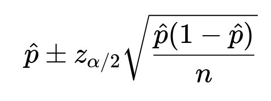
Flip the coin n times. Each flip is a Bernoulli trial with success probability p=0.6. We form a 95% confidence interval for p using the approximate formula:

Since we want the interval to exclude 0.5 from below, we set the lower bound to 0.5:

Solving for n gives approximately 93 flips.
Comprehensive Explanation

will be approximately normally distributed around the true mean p=0.6 with standard deviation

For large enough n, a 95% confidence interval for p can be approximated by


Thus, you need around 93 flips to produce a 95% confidence interval that excludes 0.5 from below when p is actually 0.6.
How to interpret this result in hypothesis testing terms

Potential Follow-up Questions
How does the number of required flips change if the coin is even more biased, say 90% heads?
If p=0.9, the difference between p and 0.5 is larger (0.4 rather than 0.1). Intuitively, you will not need as many flips to detect that the coin deviates from fairness. The step for obtaining n is similar, but the value of p(1−p) becomes 0.9×0.1=0.09 and the difference (p−0.5) becomes 0.4. Plugging these into the same style of calculation will yield a smaller n because the term under the square root is 0.09 (smaller than 0.24) and the difference (0.4) is four times bigger than 0.1, so fewer trials will be needed for the lower bound of the confidence interval to exceed 0.5.


Implementation details for verifying in code
In Python, you could simulate coin flips for a range of n and estimate the probability of rejecting p=0.5 at a 95% confidence level. For example:
import numpy as np

def coin_flips_required(true_p=0.6, significance_level=0.05, simulations=10_000):
    z_value = 1.96  # for 95% confidence
    n_candidates = range(1, 200)  # check up to 200, for example

    for n in n_candidates:
        rejections = 0
        for _ in range(simulations):
            flips = np.random.binomial(n, true_p)
            phat = flips / n
            se = np.sqrt(phat*(1-phat)/n)

            lower_bound = phat - z_value*se
            # We want the lower bound to exceed 0.5 for rejection of fairness
            if lower_bound > 0.5:
                rejections += 1

        # Check if we exceed some threshold for "confident detection"
        # e.g., we want 95% of these simulations to exclude 0.5.
        if rejections / simulations > 0.95:
            return n

    return None

needed_flips = coin_flips_required()
print(needed_flips)
This snippet uses a simulation approach. For each n from 1 to 200, it runs many simulations, constructs a 95% confidence interval around the sample proportion, and checks the fraction of times 0.5 was excluded from the interval. It returns the first n that achieves a chosen threshold of “power” against p=0.5. You would find a number in the vicinity of 90–100 flips, confirming the analytical calculation.
The main idea here is that both the analytical derivation (using the normal approximation and solving explicitly for n) and the simulation approach will converge on the same approximate range. This assures you that around 93 flips is a reasonable guideline for detecting that p=0.6 with 95% confidence.
Below are additional follow-up questions
What if the true bias is very close to 0.5, for example 0.51? How does that affect the required number of flips?

Mathematically, if the difference (p−0.5) is small, the left-hand side of the margin equation in the confidence interval approach shrinks. You might have an equation like:

If (p−0.5) is small, the required n becomes large to overcome the uncertainty from the sample variance. Practically, we can say that the more subtle the deviation from 0.5, the more evidence (i.e., flips) is needed to be sure it’s not just random fluctuation causing an estimate above or below 0.5.
A potential pitfall here is that in real-world scenarios, you might suspect a coin is “slightly loaded” (like 51%–49%), but collecting evidence to confirm it can be expensive or time-consuming. This is why, in actual applications, you often specify a “minimum effect size” (like a difference from 0.5 of at least 0.05) that you want to detect before you commit resources.
What if the coin flips are not truly independent?
The standard confidence interval and the hypothesis testing approach for a Bernoulli variable rely critically on the assumption of independence between flips. If the flips are correlated (for instance, if some external process influences consecutive flips), the variance of the sample mean changes in nontrivial ways. The Central Limit Theorem (for i.i.d. samples) does not strictly apply when there is dependency.
If there’s positive correlation—for example, if a head on one flip makes a head on the next flip slightly more likely—then the variance of the sample mean might be larger than the classical p(1−p)/n. This implies that fewer truly independent pieces of information are being obtained from each flip, so we might underestimate the number of flips required if we ignore the correlation.
A real-world illustration might be mechanical or magnetic interference in a flipping device (like a biased coin tossing machine) that causes runs of heads or tails. In that case, we need to either remove the correlation by changing the procedure or use a more advanced statistical approach (such as a generalized linear mixed model or time-series methods) that accounts for the dependency structure. Ignoring such correlation can lead to overconfidence in the interval or test result.
How should we proceed if the coin’s bias changes over time?
A varying bias over time, sometimes referred to as a nonstationary process, invalidates the assumption that each flip follows the same Bernoulli distribution with a fixed p. If the coin somehow changes its weight or if an external factor changes the flipping mechanism, the probability of heads at the i-th flip might differ from that at the j-th flip.
In such a scenario, combining all flips under one p estimate is inappropriate. The standard approach to constructing a confidence interval that assumes i.i.d. Bernoulli trials is no longer valid. Instead, you would need a model that accounts for time dependence or for changes in p(t) across different flips. This might involve:
A sliding window estimate of p that looks at recent flips only.
A model such as a hidden Markov model, where the coin bias transitions through different states over time.
Online statistical process control methods that detect shifts in probabilities.
A major pitfall is treating a changing coin as a stable coin. If you observe that your coin starts at p=0.5 but then shifts to p=0.7 mid-way, and you do not account for it, your inference about an overall p may be completely off. Hence, diagnosing stationarity before applying a Bernoulli-based method is crucial.
Could we use alternative (non-normal) approximations or exact methods, especially for smaller n?
Yes. For smaller sample sizes, the normal approximation in constructing confidence intervals is not always accurate. One can use:
The Wilson score interval, which is known to have better coverage properties than the normal approximation interval.
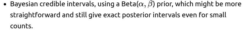
The Clopper–Pearson interval, an exact confidence interval based on the Beta distribution, which can be more conservative but provides guaranteed coverage.

A subtle pitfall with the classical normal approximation method is that it can produce poor estimates when n is small or p is extremely near 0 or 1, potentially leading to confidence bounds outside [0,1]. If your sample size is under, say, 30 flips, it’s often advisable to consider exact intervals or at least the Wilson interval to avoid those boundary issues.
What if we want a specific statistical power (e.g., 80% or 90%) to detect a difference from 0.5?
In hypothesis testing, the term “power” refers to the probability of correctly rejecting the null hypothesis when the alternative is true (i.e., a true difference exists). Having 95% confidence focuses on your Type I error rate (chance of falsely rejecting a true null), but it doesn’t directly address power. If you want, say, 80% power to detect a difference of 0.1 (from 0.5 to 0.6), you need to solve a power analysis equation:

The pitfall here is that some might conflate “confidence level” with “power.” They are two different quantities. A 95% confidence level sets how often you’re wrong when p is actually 0.5, while power sets how likely you are to detect a difference of 0.1 (if it truly exists). If you do not conduct a proper power analysis, you might incorrectly conclude a small sample size suffices, only to find you frequently fail to detect the real difference.

Are there any issues if the observed proportion is exactly 0 or 1 in initial flips?
Yes, this situation can arise if, by chance, all the first few flips come out the same. For example, if the first 10 flips are all heads, you might get a naive confidence interval that suggests p=1.0 with no variation, which is obviously an extreme estimate. In the strict sense, a normal approximation for a single sample proportion of 1.0 will give you zero for the standard deviation, leading to an unbounded scenario or degenerate intervals.
In a real-world scenario with small n, exact methods or the Wilson interval (and Bayesian methods) handle this more gracefully because they avoid producing degenerate estimates. For instance, the Wilson interval will never produce exactly 0 or 1 as its endpoints (assuming a finite sample), and a Beta prior in a Bayesian framework will ensure the posterior never places all its mass on 0 or 1 unless you have an extremely strong prior or infinite flips.
Hence, a major pitfall in practical applications is ignoring or mishandling the scenario where you see all heads or all tails in a small sample. It’s best to adopt an interval estimation method that is robust to such edge cases.
How could small sample corrections, like the continuity correction, change the required flips?

For instance, you might adjust a test statistic by adding or subtracting 0.5/n when shifting from discrete counts to a continuous approximation. This can affect the number of flips needed, especially when n is borderline for the normal approximation. While for large n this effect becomes negligible, for moderately sized n, such as around 30, 40, or 50, it can make your confidence intervals and test decisions more accurate. Ignoring continuity correction might lead you to underestimate or overestimate the confidence bounds for p.
A pitfall is that many textbooks omit the continuity correction because it complicates formulas and is less relevant with big data. But in an interview scenario, you should at least be aware that normal approximations to binomial counts can be improved for moderate sample sizes by applying small corrections.
Does the same methodology apply if we have multiple coins to compare?

One subtlety is that you need to control for multiple comparisons if you are testing multiple coins or multiple hypotheses about the same coin. For example, if you test 10 coins for fairness at the 95% confidence level without adjusting for multiple testing, your chance of making at least one Type I error (falsely rejecting fairness) rises above 5%. A more rigorous approach is to use procedures like the Bonferroni correction or the Holm method to maintain an overall significance level.
Pitfalls here include inflated false discovery rates when testing many coins, not pooling variance estimates correctly, or ignoring that the total number of flips might be allocated differently among the coins.
How do practical considerations, like cost or time constraints, affect the choice of “how many flips”?
In real-world applications, you may not simply optimize for statistical rigor. You also have a budget constraint (e.g., each flip is an expensive physical experiment) or a time limit. You might decide to settle for a lower power or confidence level to reduce the number of flips. Alternatively, you might run a sequential test, deciding after each flip whether you have enough evidence to reject p=0.5 or to continue flipping.
This highlights a major real-world pitfall: purely statistical solutions might say “we need 1,000 flips to be sure.” But if collecting 1,000 flips is not possible or is prohibitively costly, you have to strike a balance between how certain you want to be versus how much you can afford to collect data. The field of sequential analysis can help optimize how many flips to do on-the-fly, making the problem more flexible to constraints like cost or time.