
ML Interview Q Series: Detecting Concept Drift via Monitoring and Adapting Models with Retraining/Online Learning
📚 Browse the full ML Interview series here.
Concept Drift: Over time, the data going into your deployed model starts to differ from the data it was trained on – a situation known as concept drift. How would you detect that concept drift is occurring, and what actions could you take in response to maintain your model’s performance? *Include ideas like monitoring model predictions vs actuals, statistical tests on input feature distributions over time, and strategies like periodic retraining or online learning.*
Detecting and responding to concept drift is essential for real-world machine learning systems. When a model is deployed, the assumptions made at training time may gradually or abruptly become invalid as the data distribution shifts. This can significantly degrade model performance if not addressed. Below is a detailed discussion of how to detect concept drift, followed by potential actions to maintain model performance. Then we delve into probable tricky follow-up questions and answer them in depth.
Understanding Concept Drift
Concept drift occurs when the relationship between input features and target labels changes over time. This can take different forms, often categorized as real concept drift (the true relationship changes), virtual drift (the distribution of features changes even if the underlying relationship might not), or sudden vs. gradual drift. In practice, these distinctions help guide what monitoring strategies to use and how to adapt your model.
Detecting Concept Drift
Monitoring Predictions vs Actuals
Observing a degradation in typical performance metrics (such as accuracy, F1-score, or RMSE) on recent data can indicate drift. If you have access to ground truth labels (even with some delay), you can compute how the model’s predictions deviate from the actual outcomes over time. A steady decline in performance is often the first sign of concept drift.
Evaluation on a Holdout or Rolling Window A rolling window approach involves periodically retraining and evaluating the model on recent batches of data. By tracking performance metrics on each new window, unusual drops can signal drift. This approach is particularly useful when you have a continuous flow of time-stamped data.
Statistical Tests on Feature Distributions
Features can shift in distribution. You can perform distribution tests to see if the new data differs statistically from older (training) data. There are many possible tests, including the two-sample Kolmogorov–Smirnov test, the Wasserstein distance, or the Kullback–Leibler divergence.
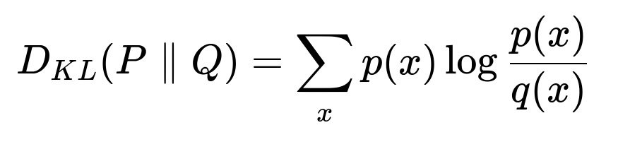
In the above expression, p(x) can represent the probability distribution of a feature during training, while q(x) represents the probability distribution of the same feature on newly incoming data. A significant divergence indicates that the feature distribution has shifted. Similarly, for continuous distributions, integral or density-based forms would be used. While each measure has its nuances, their general goal is to detect distribution changes over time.
Unsupervised Drift Detection
Unsupervised methods do not rely on label availability. You can embed incoming data in a latent space and use clustering or reconstruction errors to detect when incoming samples are outliers relative to the training data distribution. Autoencoders can be employed: if the reconstruction error for new data is significantly higher than during training, it might suggest that the underlying data distribution has shifted.
Actions to Maintain Model Performance
Periodic Retraining
Periodically retraining the model on fresh data is a straightforward approach. This can involve: Retraining from scratch with all historical data plus a buffer of the newest data. Fine-tuning the existing model with a sliding window of the most recent data. Either strategy ensures that the model parameters get updated to reflect new trends. However, these approaches can be computationally expensive and should be scheduled wisely based on the rate of drift and costs of retraining.
Online Learning
Online (incremental) learning updates model weights on-the-fly as new samples arrive. This approach is particularly common for streaming data scenarios, where data arrives continuously. Algorithms like Stochastic Gradient Descent or specialized online algorithms can incorporate each sample (or mini-batch) as soon as it is available. Online learning can adapt more rapidly to evolving distributions but requires careful hyperparameter tuning to avoid forgetting past knowledge too quickly.
Adaptive Ensemble Methods
Ensemble techniques can be used to maintain multiple models, each trained on different temporal segments of the data or under different conditions. New data can be used to add or remove ensemble members. Methods such as online boosting or online bagging adapt to new data by re-weighting ensemble members in proportion to their performance on recent samples.
Data-level Interventions
If concept drift is caused by external factors that can be addressed at the data-collection level, you might introduce new features, remove outdated features, or filter out anomalous data points to align your input distribution closer to the new reality. This helps keep the model relevant even before re-training.
Extensive Validation Pipelines
Set up a robust pipeline to continuously validate the model on both: A stable test set reflecting older distributions (to measure performance on the original concept). A streaming or recent test set capturing the latest data. Significant discrepancies between these two validation sets can highlight drift.
Model Agnostic Correction Layers
You can have a “correction” layer on top of the core model, retrained more frequently than the main model, effectively learning the new offsets or biases. This layer might take the outputs of the main model plus recent feature statistics as input, then correct or calibrate the final prediction.
Code Example for Detecting Feature Distribution Changes in Python
import numpy as np
import scipy.stats as stats

# Suppose old_data and new_data are numpy arrays representing a single feature
# or some projected dimension in a latent space.

# Perform a two-sample Kolmogorov–Smirnov test
statistic, p_value = stats.ks_2samp(old_data, new_data)

if p_value < 0.05:  # using a significance level
    print("Distribution shift detected for this feature (p-value < 0.05).")
else:
    print("No significant distribution shift detected (p-value >= 0.05).")
Such statistical tests can be performed feature by feature or on reduced-dimensional embeddings to detect overall distribution changes.
How would you handle delayed ground truth when trying to detect drift?
When labels arrive with a delay, it is impossible to immediately measure prediction vs. actual performance. One approach is to keep a buffer of predictions and, once the labels become available, align them with their corresponding predictions to compute delayed performance metrics. Meanwhile, unsupervised drift detection on input features can still be used to monitor potential drift in the absence of current labels. Once the delayed labels come in, you can update performance measures and confirm whether the drift is real concept drift (target distribution change) or merely changes in input distribution that may not affect the outcome.
If the delay is very large, you may rely heavily on unsupervised or semi-supervised drift detection and only periodically refresh model parameters when enough labeled data becomes available to confirm drift has occurred.
What if the data distribution changes suddenly rather than gradually?
Sudden or abrupt drift occurs if there is a major event (for example, a financial crash or a change in user behavior pattern). In this scenario, a previously well-performing model might fail almost overnight. Detecting this requires real-time or near-real-time monitoring of input feature distribution or model performance metrics. Early warning mechanisms, such as a statistical process control chart or a threshold-based system on feature distribution distances, can trigger an emergency retraining pipeline or failover to a simpler rule-based system while a new model is quickly re-trained.
Are there specialized algorithms for handling concept drift in streaming data?
Many algorithms specifically address streaming data with concept drift: Incremental decision trees (e.g., Hoeffding Trees) that can grow or prune branches based on new information. Online gradient descent methods that continuously update weights. Drift detection methods like Drift Detection Method (DDM) or Early Drift Detection Method (EDDM) that examine changes in error rate. Adaptive sliding window strategies that keep only recent data for training.
The goal is to adapt to the new distribution while minimizing catastrophic forgetting of older concepts that might still be relevant.
How do you decide between retraining from scratch vs. fine-tuning with new data?
Retraining from scratch is more computationally expensive and might cause the model to “forget” older patterns if the older data is not included. It can be beneficial if: The feature distribution has changed dramatically and the old data is no longer relevant. You have access to a large pool of historical data to combine with new data and can afford to train a new model.
Fine-tuning or incremental updates are preferable if: The core representation remains valid and only partial corrections are needed. You want to quickly incorporate new data without heavy computational costs. Both approaches can be combined: maintain a rolling buffer of data from different time periods, and either fine-tune the model or occasionally retrain from scratch using the entire buffer to avoid excessive drift or catastrophic forgetting.
How can you maintain model performance when you have very limited new data?
In scenarios where you receive only a small amount of new data, methods such as: Few-shot learning or meta-learning approaches that quickly adapt to small distribution changes. Transfer learning techniques where you keep most of the original model weights fixed and adjust only a small number of parameters. Regularization strategies that constrain large shifts away from the original weights.
You might also employ data augmentation or synthetic data generation if feasible. The core idea is to balance old knowledge with minimal new data, carefully updating the model in a stable manner.
How do you handle the case where concept drift is cyclical?
Cyclical or seasonal drift occurs when data distribution repeats a pattern periodically (like daily, weekly, or yearly cycles). The best approach is to incorporate known seasonal features into the model and keep track of these cyclical patterns. You can maintain multiple models for different seasons or use a single model augmented with time-related features so it can learn the periodic behavior. Carefully curated validation sets that mimic the cycle can reveal whether your model is capturing these recurring patterns. Furthermore, a robust pipeline that re-checks performance every cycle boundary is crucial to ensure consistent accuracy.
Why might an ensemble approach help more than a single model in the face of drift?
An ensemble of models that each specialize in different time periods or data regimes can be more robust to drift. As new data arrives, you can measure which ensemble member performs best on fresh batches. Older ensemble members can be pruned or down-weighted if they consistently underperform. This dynamic weighting or pruning mechanism allows the system to smoothly transition to the model or set of models that are most in sync with the current data distribution. Ensemble diversity also reduces the risk that a single model’s biases dominate and degrade performance under drift.
Are there any risks or pitfalls when continuously updating a model in production?
A key pitfall is catastrophic forgetting: if you constantly update with only the most recent data, you risk discarding useful patterns learned from historical data. This is especially problematic if the distribution oscillates or returns to a prior state later. You also risk reacting to temporary noise in the data and incorporating spurious patterns, leading to instability. Another common issue is label leakage or data contamination: if not handled carefully, you might include wrongly labeled data or data that is not representative of the actual distribution.
Hence, deploying an online learning system should be done with guardrails, such as stable test sets, clear drift detection thresholds, safe fallback models, and thorough logging of changes.
How would you design a monitoring system to detect drift in an enterprise-scale application?
You would create a pipeline that collects real-time or near-real-time data on: Statistical summaries of input features (mean, variance, histograms, etc.). Model performance metrics on recent labeled data (when available). Distribution shift metrics such as KL divergence or Wasserstein distance between old and new features.
You would store these metrics in a time-series database to enable anomaly detection or threshold-based alerts when drift surpasses certain levels. You could set up dashboards for data scientists and stakeholders to visualize drift trends over time, allowing them to intervene as soon as drift is detected.
If you maintain a robust DevOps or MLOps setup, you might automatically trigger a new training job or switch traffic to a shadow model upon drift detection. This system must be thoroughly tested to ensure that it doesn’t overwhelm teams with false positives and that it can rapidly detect real drift.
What if the ground truth itself changes definition over time?
Sometimes the definition of the label or the “true” concept can evolve. This is more than a mere distribution shift; it may require re-labeling historical data or recalibrating the model. For instance, in a fraud detection system, the definition of “fraudulent” transactions can shift with new regulations or new attacker behaviors. In these cases, you might need to re-collect or re-annotate data that fits the new definition to train a model that aligns with the changed label semantics. This underscores the importance of version-controlling both your datasets and label definitions to handle changes in the fundamental concept being modeled.
Could bandit or reinforcement learning approaches help?
Yes, if you have a setting where you can experiment and collect immediate feedback (like click-through data in a recommender system), multi-armed bandit or reinforcement learning algorithms can continuously adapt to new user behavior. These algorithms inherently handle a constantly changing reward distribution by exploring new actions and exploiting known good actions. They can detect shifts in reward patterns (i.e., user responses) relatively quickly, reassigning preference weights to actions that yield higher reward under the new environment.
How does one validate a new model if drift is continuous?
Traditional train/test splits become less meaningful when the data distribution keeps shifting. A robust approach involves: Temporal cross-validation or rolling window evaluation. Segmenting data into time-ordered chunks, training on one chunk, and validating on the immediate next chunk to simulate real deployment. Continuously measuring error metrics in a sliding window manner. This ensures your evaluation results remain aligned with the most current data distribution, providing a realistic measure of how well the model will perform as it’s deployed.
How can you ensure fairness and bias mitigation under drift?
If you have fairness constraints or want to ensure the model is not discriminating against certain subgroups, you must monitor fairness metrics (like demographic parity or equalized odds) continuously. Concept drift might disproportionately affect certain subgroups, even if it doesn’t affect the overall distribution equally. Tools exist for measuring subgroup performance over time. If you see that certain protected classes are suddenly experiencing degraded performance, it might indicate a subgroup-specific drift, prompting targeted retraining or data collection to keep the model fair.
Below are additional follow-up questions
How would you detect and handle drift when the model’s predicted output distribution remains stable, but individual features exhibit shifting relationships to the target?
When concept drift occurs, sometimes the aggregate output distribution (e.g., the fraction of positive vs. negative predictions) might look stable, so basic monitoring of prediction rates might not detect a problem. However, certain features could start interacting with the target differently, causing “hidden” drift that might only reveal itself in more granular metrics.
One approach is to track feature-target relationship statistics over time. For a categorical variable, you can group data by category and check how often each category is correctly predicted. For continuous variables, you might bucket or discretize them and look at metrics within each bin. If, for example, a feature bin used to have a high conversion rate but that rate is dropping while the overall conversion rate remains constant, that indicates local drift. A detailed approach might involve:
Computing a confusion matrix stratified by different feature ranges or categories.
Tracking feature importance changes in a model-agnostic manner (e.g., using a permutation-based method) on separate time slices.
Employing partial dependence or SHAP value analysis periodically to see if a feature’s marginal contribution changes dramatically.
A potential pitfall is missing this drift if you only track overall metrics like accuracy or AUC. Those metrics can stay constant if the positive/negative label ratio in the data remains stable, even while the underlying decision boundaries have shifted. This can lead to unexpected performance degradation on certain subgroups or feature regions, which only becomes obvious once you break down the data more granularly.
How can you prioritize which features to monitor for concept drift in a high-dimensional data scenario?
In very high-dimensional data, monitoring every feature individually can be expensive computationally and cognitively overwhelming. You need a strategy to decide which features (or sets of features) are most critical to track:
Feature Importance: You can rank features based on their importance during model training (using methods like Gini importance for tree-based models or weight magnitudes for linear models) and focus on the top features.
Variance Threshold: Features that historically exhibit higher variance in their values are more prone to distribution shifts. Low-variance features typically remain stable.
External Domain Knowledge: If subject-matter experts know certain features are more susceptible to temporal or external changes, prioritize those for drift monitoring.
Dimensionality Reduction: You can monitor drift in a lower-dimensional latent representation (e.g., PCA or autoencoder embeddings). If the embedding distribution shifts, it could signal broader changes in the original feature space.
A potential edge case arises when a feature that was previously less important becomes more relevant due to a shift in the environment. Relying exclusively on past importance or variance could miss this scenario. To mitigate that, a combined approach—feature importance plus periodic checks of distribution changes in lower-dimensional embeddings—helps catch unexpected drift in seemingly minor features.
What if part of your data experiences drift while another subset remains stable, and you still want to maintain a single global model?
This selective or localized drift can occur if only certain segments of your user base or certain product categories change behavior. If you maintain just one global model, it might degrade overall while still performing acceptably on unaffected segments. However, ignoring this localized drift risks losing performance in the changed segments.
To handle this scenario under a single global model approach, you can:
Segment-Based Analysis: Periodically group data into segments that might be subject to different behaviors (e.g., user demographics, product categories) and analyze performance within each segment.
Adaptive Loss Weighting: If certain segments are drifting more quickly, you can upweight those examples in your training or fine-tuning to ensure the model devotes enough capacity to learning the new patterns.
Hybrid Approaches: You might create specialized “expert” sub-models for each drift-prone segment, then combine their outputs within a single global model pipeline.
A subtle pitfall is allowing the global model to degrade on stable segments while overly focusing on the drifted segments. Continuous monitoring of performance across segments and an overall measure ensures you preserve performance across the entire distribution.
How do you handle concept drift in a system where the model’s inference speed and latency requirements are extremely strict (e.g., high-frequency trading or real-time bidding)?
In latency-sensitive applications, re-training or updating a model must be balanced against the disruption and computational overhead. Some strategies include:
Lightweight Online Updating: Incrementally update a small subset of model parameters or a simpler proxy model instead of re-training a deep or complex model from scratch. This can keep real-time inference pipelines intact.
Shadow Models: Train a new model (or set of candidate models) offline while the current model is serving requests. Then, once the new model is ready and tested, do a switchover with minimal downtime.
Compressed or Quantized Models: If concept drift requires deploying new models frequently, keep models small (quantization, pruning) for faster redeployment and lower memory footprint.
Feature and Model Caching: Maintain a queue of recent data and apply updates in micro-batches if purely streaming updates cause too much overhead. This trades off some responsiveness for stability.
A potential edge case is if drift happens so fast that even a small delay in updating the model can lead to huge losses (financial, user experience, etc.). In that case, more advanced approaches, such as streaming-friendly algorithms with constant time/space updates, might be required. The risk is that these extremely adaptive models can overfit quickly to transient noise in the data.
Could active learning approaches help manage concept drift more efficiently?
Active learning can be particularly helpful if labeling is expensive, and you have streaming or continuous data. The model selectively queries labels for the most “informative” or “uncertain” new samples. This helps maintain model performance under drift by focusing labeling efforts on areas where the model is likely to be wrong.
For instance, if the model suddenly shows high uncertainty or surprising predictions for a subset of new data, that suggests a potential distribution shift. By actively querying labels in that region, you can confirm drift and retrain only if necessary.
A subtle issue arises if the drift is silent (the model’s confidence remains high even as data shifts). In such cases, you might not realize you need to query new labels. A fallback is to incorporate an unsupervised drift detector that monitors feature distributions, triggering active queries when suspicious changes appear. You must also ensure your active learning strategy doesn’t repeatedly oversample only the newly drifted region and forget about stable segments.
How do you handle the risk of data privacy violations when continuously collecting data for drift detection in sensitive domains?
In highly regulated industries (healthcare, finance), data collection and drift monitoring must comply with strict privacy requirements. Approaches to mitigate privacy risks include:
Aggregation and Anonymization: Monitoring distribution statistics (e.g., average, variance, correlation) at an aggregate level rather than collecting individual records in plain form.
Differential Privacy: Adding controlled noise to your drift metrics so individual data points cannot be traced.
Federated Learning: Keeping data on local devices or local servers and only sharing minimal, encrypted updates with a central server.
Synthetic or Summarized Data: If you need to analyze the distribution, you might generate synthetic data that approximates the real distribution but does not reveal private details about actual individuals.
A pitfall is believing that simple aggregation automatically solves privacy. In small subgroups, it might still be possible to re-identify individuals if the system is not carefully designed. You also need to ensure that any drift detection approach that uses raw records is thoroughly audited. A robust compliance check with privacy officers or legal counsel is standard practice in sensitive domains.
When would you choose to adopt a specialized “domain adaptation” technique instead of typical retraining or online learning for drift?
Domain adaptation techniques are especially powerful if you have a well-labeled “source” domain (original training environment) and a differently distributed “target” domain (new environment) with few or no labels. Classical retraining or online learning would require more labels in the new domain. Domain adaptation, however, can leverage the source data and any structural similarities between the source and target to adapt the model effectively with minimal new labeling.
For instance, if you developed a sentiment analysis model on social media posts in one language or region but want to apply it to another region with slightly different linguistic patterns, domain adaptation methods can refine representation layers to handle that shift without requiring full re-labeling. Pitfalls include:
Assuming the “shift” can be well-aligned by simply matching feature distributions without verifying the label semantics remain consistent. If the fundamental label definition changes, domain adaptation might fail.
Overly relying on unsupervised domain adaptation, which can adapt to differences in feature distribution but not necessarily account for changes in the meaning of the label itself.
In a multi-task or multi-objective setting, how do you deal with the possibility that some tasks drift while others remain stable?
When you train a single model to address multiple tasks (e.g., multi-task learning), concept drift can affect tasks unevenly. For example, in an autonomous driving scenario, the object detection module might drift if new types of objects appear, while lane detection remains stable. You have choices:
Task-Specific Monitoring: Track performance metrics individually for each task, possibly with separate drift detection frameworks.
Selective Retraining: Update only the task head or loss weighting for the drifting task, while preserving the others if they remain stable.
Decoupled Architectures: If tasks share some backbone layers, consider a small set of parameters dedicated to each task. That way, you can fine-tune or adapt only the subset relevant to the drifting task.
A subtle edge case is that changes in one task’s data might indirectly affect the features or representations used by other tasks. Ensuring you do not degrade stable tasks while improving the drifting task requires thorough cross-validation across all tasks after any adaptation.
What if concept drift is intentionally introduced, such as when you change the feature engineering pipeline in production?
Sometimes, data drift isn’t external but arises because of internal changes: you might modify how data is aggregated, apply new transformations, or roll out a new sensor. This can abruptly shift feature distributions. In such cases:
Versioning the Data Pipeline: Always track which version of the feature engineering code produced which dataset. If a performance drop or drift alert triggers, confirm if it correlates with pipeline updates.
Feature Mapping or Alignment: If the new pipeline yields a feature that doesn’t map one-to-one to the old pipeline’s feature, you may need a calibration or mapping function that translates old feature values to new ones, ensuring continuity.
Gradual Rollout: Run both old and new pipelines in parallel (“shadow mode”) for a short period to gather data and confirm that the new features remain compatible with your model.
An edge case is if the old pipeline had hidden data-leakage or certain biases that have now disappeared in the new pipeline. The model might see a performance drop simply because the new pipeline is actually more correct. Careful analysis can distinguish beneficial “removal of bias” from detrimental “feature mismatch.”
How do you maintain interpretability and trust with stakeholders when the model is continuously adapting to drift?
In many business or regulated contexts, stakeholders need to understand and trust the model’s decisions. Continuous adaptation can be unsettling if the reasons behind each update are not clear. Possible solutions:
Model Cards and Update Logs: Document each time you retrain or update the model, specifying why it was done (e.g., performance drop, detected drift) and summarizing the changes in performance or distribution.
Explainable Surrogates: Use an interpretable model (like a small decision tree or rule list) as a local surrogate to show approximate changes in how predictions are made after updates.
Human-in-the-Loop Checkpoints: Before finalizing a new model update, generate interpretability reports that highlight how feature importance or partial dependence has changed. Let domain experts sign off if the changes align with known real-world shifts.
A subtle pitfall is that frequent updates might produce contradictory explanations over time. The system should track how major interpretability metrics shift across versions, so you can provide a historical narrative: “As the data environment changed, the model started to rely more on feature A and less on feature B, which aligns with event X in the real world.”
What if drift occurs in an unsupervised setting (no labeled data), such that there is no concept of “correctness” in the classical sense?
In purely unsupervised systems (like anomaly detection or recommender systems without explicit labels), “concept drift” refers to changes in the underlying data distribution or user behaviors that cause the model’s learned representation or clustering to become outdated. Potential actions:
Periodic Reconstruction Error Checks: If you use an autoencoder or other dimensionality reduction technique, monitor reconstruction error over time. A rise might suggest new data points no longer look like the training distribution.
Cluster Purity Measures Over Time: If you cluster data, you can track how stable or cohesive those clusters remain as new data arrives. A cluster splitting or merging unexpectedly might signal drift.
User Feedback Loops: In recommendation systems, user interactions (like clicks or dwell time) can act as a proxy label. If user engagement drops for certain recommended items, it may indicate drift.
An edge case is that changes in reconstruction error might be caused by natural periodic variations rather than drift. This highlights the importance of looking for consistent trends rather than single spikes. You must also ensure your drift detection method in unsupervised settings does not conflate outliers with genuine distribution shifts.
Is it ever acceptable to allow a model to operate for a while in a “degraded” state before reacting to drift?
Depending on the cost of incorrect predictions versus the cost of frequent retraining, some organizations may tolerate a temporary decrease in performance. For instance, if retraining is extremely resource-intensive or if the user impact of the error is small, you might let the model degrade slightly for a limited period. You can then schedule updates at more optimal times:
Graceful Degradation Thresholds: Define acceptable performance bounds (e.g., accuracy must not drop below a certain threshold). Only trigger re-training if it goes below that threshold consistently.
Retrain Windows: Have a planned schedule (e.g., weekly or monthly) unless performance catastrophically fails.
However, a tricky edge case is if drift is extremely fast and large in magnitude. The model might degrade severely before the next scheduled retrain. This can have severe consequences in certain domains (safety-critical or high-value financial transactions). So organizations must weigh the operational cost versus the risk of wrong predictions to decide the acceptable window for being in a degraded state.
How might you automate the entire drift detection and remediation pipeline?
Large-scale industrial systems often rely on an automated MLOps or DataOps pipeline:
Data Ingestion: Gather real-time or batch data, log model inputs and outputs.
Monitoring Service: Compute distribution statistics, performance metrics (if labels are available), and drift detection metrics on a schedule or in real-time.
Alerting Mechanism: When drift or performance degradation surpasses predetermined thresholds, trigger alerts.
Automated Model Training: If the alert system indicates a serious shift, automatically spin up a new training job using the latest data.
Continuous Deployment: Deploy the newly trained model in a staged environment, run A/B tests or canary deployments, and if everything looks good, roll out to production.
A potential pitfall in fully automated pipelines is “alert fatigue” or “model churn” if the thresholds are set too low. That might cause constant retraining on minor variations, resulting in overhead and potential instability. Carefully designed thresholds, plus manual oversight or gating steps, help strike a balance between agility and stability.