
ML Interview Q Series: Detecting Unfair Coin Bias: Sample Size Calculation via Hypothesis Testing

Browse all the Probability Interview Questions here.
11. Say you have an unfair coin which will land on heads 60% of the time. How many coin flips are needed to detect that the coin is unfair?
Understanding the question in a rigorous way involves classical statistical hypothesis testing. We want to know the sample size (number of coin flips) required so that, with high probability, we can conclude the coin's true probability of landing heads is 0.6 (as opposed to the fair coin assumption of 0.5). This typically means setting up a null hypothesis that the coin is fair (p = 0.5) and an alternative hypothesis that p ≠ 0.5 or p > 0.5. We then specify a significance level (often denoted

) and a desired statistical power (often denoted
1−β
). Once these are fixed, we can estimate the required number of coin flips using well-known formulas or direct simulation.
Detecting “unfairness” precisely depends on thresholds for statistical significance (the probability of a Type I error, rejecting a fair coin when it is actually fair) and power (the probability of detecting that the coin is unfair when it is indeed biased). Although there is no single universal answer unless we specify these thresholds, it is standard to assume something like a 5% Type I error rate (

) and 80% power (
1−β=0.80
). Under these assumptions, the required sample size to detect a shift from p = 0.5 to p = 0.6 often falls roughly in the ballpark of 100–200 flips. We will walk through the reasoning and provide a more precise normal-approximation-based calculation below.
Hypothesis Testing Approach
First, to set up the hypothesis test, we consider:
Null hypothesis

Alternative hypothesis

(or more generally p ≠ 0.5)

We want to control the probability of a false alarm (Type I error) at

. We also want a reasonable probability (power)
1−β
of detecting the difference p = 0.6 from p = 0.5 if it truly exists (often power is set at 0.80 or 0.90).
Using a Normal Approximation
A common way to approximate the number of required coin flips n is via the normal approximation to the binomial distribution. For a single-proportion z-test, we can use a formula that takes into account both the significance level

and the power
1−β
. Denote:
ParseError: KaTeX parse error: Can't use function '$' in math mode at position 17: …_{1 - \alpha/2}$̲$ as the critic…
Under the null hypothesis, we assume p = 0.5 with variance 0.5 * 0.5 = 0.25. Under the alternative, p = 0.6 with variance 0.6 * 0.4 = 0.24. A commonly used form of the sample size formula for detecting a difference between two proportions p₀ and p₁ is adapted here for the special case of p₀ = 0.5 and p₁ = 0.6:

Substitute p₀ = 0.5, p₁ = 0.6,

Hence
n≈194
coin flips. This is under typical assumptions of a two-sided test at 5% significance and 80% power. If you wanted a one-sided test (for instance, you suspect p > 0.5, not just p ≠ 0.5), the value of

might be replaced by

, leading to a slightly smaller required n. If you demanded a higher power like 0.90 or a stricter significance like

, the required n would increase.
Simpler Approximation for Rough Estimation
Another simpler approach is to treat 0.5 as the center of a normal distribution with standard error
. Under p = 0.5, that standard error becomes

. If we want to detect a shift of 0.1 (from 0.5 to 0.6) at roughly 2 standard errors (for a quick approximate 95% confidence region), we would solve:

Which simplifies to:

Hence

So
This is a rough estimate ignoring power in a formal sense, but it gives the general scale that around 100 coin flips might often be enough to demonstrate unfairness. A more precise calculation, as shown earlier, usually yields a slightly higher value when we strictly enforce both a 5% false alarm rate and 80% power.
Practical Simulation Approach
A data-driven practitioner might prefer running a simulation to see how many coin flips it takes, on average, to reject the fair coin hypothesis when the coin is actually p = 0.6. Below is an illustrative Python snippet that simulates repeated experiments, each with a certain number of flips, to see how often we correctly conclude the coin is not fair:
import numpy as np
from statsmodels.stats.proportion import proportions_ztest

def simulation_unfair_coin_detection(num_flips, prob_heads=0.6, alpha=0.05, trials=100000):
    rejections = 0
    for _ in range(trials):
        flips = np.random.rand(num_flips) < prob_heads
        heads_count = flips.sum()
        # We do a 2-sided test: H0: p=0.5, H1: p != 0.5
        # proportions_ztest expects count of "successes" and sample size
        stat, pval = proportions_ztest(heads_count, num_flips, value=0.5, alternative='two-sided')
        if pval < alpha:
            rejections += 1
    return rejections / trials

# Example usage: check detection rate for different n
for n in [50, 100, 150, 200]:
    power_est = simulation_unfair_coin_detection(n)
    print(f"{n} flips -> Estimated power = {power_est:.3f}")
In this simulation:
We generate Bernoulli trials with success probability p = 0.6.
We do a two-sided test at

for the hypothesis p = 0.5.
We see how frequently we reject the null hypothesis. This frequency is our estimate of the power (probability of detection).
As we increase the number of flips n, we expect the power to approach 1, meaning it becomes very likely we detect the coin is biased.

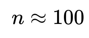
You would typically see that around n = 100 or n = 150, the power becomes meaningfully high to detect the difference between 0.6 and 0.5.
Confidence Intervals as Another View
Instead of a hypothesis test, you can look at the 95% confidence interval for the estimated probability of heads. If the coin is truly 0.6, your observed sample proportion after n flips is likely (though not guaranteed) to be near 0.6. Once that observed estimate is sufficiently different from 0.5 in a statistically significant way, you can say that 0.5 no longer lies within your confidence interval. In practice, the length of the confidence interval shrinks roughly with
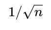
, so the more flips, the more precisely you can pinpoint the coin’s bias.
Real-World Considerations
There are subtle issues:
If we use a two-sided test, we might “waste” some significance on the possibility that the coin is p < 0.5, even if we strongly suspect p > 0.5. If we use a one-sided test p > 0.5, we can reduce the sample size a bit. But if the real coin were biased to p < 0.5, a one-sided test might fail to detect that.
If we require extremely high confidence (e.g.,

) or extremely high power (e.g., 99%), the number of required flips can become quite large, often in the hundreds or more.
If the coin’s bias were less pronounced (say 0.52 vs. 0.5), many more flips would be required.
If the coin is subject to mechanical or environmental changes during flipping (e.g., changes in flick strength or environment), the assumption of identical and independent flips might be violated.

Summary of the Core Idea
In general, to detect a moderate bias of 0.6 with a standard 5% significance and 80% power, you often need on the order of 100–200 coin flips. A more precise calculation via the normal approximation to the binomial distribution typically yields around 190–200 flips for a strict two-sided test with the above parameters, but a simpler approximate rule suggests that around 100 flips is often enough to at least start to see evidence of bias.
What if the interviewer asks: “Why is there no single universal answer without specifying the significance level and power?”
A direct reason is that statistical hypothesis testing always involves controlling two types of errors: Type I (false positives) and Type II (false negatives). Significance level

controls the maximum allowed probability of a false positive (concluding the coin is unfair when it is actually fair). Power
1−β
controls how likely we are to detect the unfairness if it truly exists. Depending on how strictly or loosely one sets

and
β
, the required sample size changes. Without clarifying these criteria, any number we quote is missing an essential part of the problem’s specification.
The significance level and power reflect real-world trade-offs. In a real experiment, you might accept a higher chance of a false positive if you need fewer coin flips. Or you might be more cautious and set

to be extremely small. The question’s answer heavily depends on these parameters. That is why standard practice is to fix them (commonly

and power = 80%) to get a recommended range of n.
What if the interviewer then asks: “Why use a normal approximation rather than the exact binomial test?”
Using the exact binomial test is more accurate for small samples because it does not rely on the asymptotic normal distribution assumption. However, for large n, the binomial distribution can be approximated quite well by a normal distribution under the Central Limit Theorem. The normal approximation offers closed-form formulas for quick estimates, making it easy to solve for n explicitly. If n is small, you can do an exact computation or rely on tables or iterative methods. In practice, for sample sizes above roughly 30–40 flips, the normal approximation is often quite reasonable for a quick calculation, though modern statistical packages can handle the exact binomial test easily.
What if the interviewer challenges: “What if your real estimate after n flips is not exactly 0.6 but something slightly below or above?”
Random sampling error means we typically won’t get exactly the true p in our sample proportion. Even if the coin is truly p = 0.6, the empirical proportion in a finite sample might be 0.57, 0.63, 0.64, 0.54, and so on. What truly matters is whether our observed result is sufficiently far from 0.5 to reject the hypothesis that p = 0.5. The larger n is, the smaller the standard error of the sample proportion, and the easier it is to conclude that 0.6 is not 0.5.
If in a given sample of n flips we get an empirical proportion

that’s close to 0.5, we might fail to reject the null hypothesis for that particular experiment. However, as n grows and we keep seeing about 60% heads overall, the test statistic will drift away from 0.5 in a more consistently significant way.
Potential Pitfalls and Real-World Nuances
One subtlety is that the coin flips must be i.i.d. (independent and identically distributed). If flipping mechanisms or flipping strength change over time, or if the coin gets physically altered, the distribution might shift. Another subtlety is p-hacking or repeated significance testing. If someone flips the coin 10 times, sees 6 heads, claims significance, flips more times, etc., the procedure becomes complicated because repeated inferences inflate the false positive rate.
In a real setting, you must define in advance how many coin flips you plan to do and what test you will apply. This pre-specification is the standard approach in well-designed experiments to ensure valid p-values.
Conclusion of the Discussion
By setting typical standards for significance (

) and power (
1−β=0.8
), we arrive at roughly 100–200 coin flips required to detect the difference between p = 0.5 and p = 0.6 with a reasonably high chance of success. A more exact normal-approximation-based formula yields close to 194 flips for a two-sided test at 5% significance with 80% power. However, around 100 flips is often a good rough estimate to begin seeing a statistically significant bias if the true probability is 0.6. Once you specify all your testing parameters (exact or approximate test, one-sided or two-sided, your

and
β
), the sample size question can be answered precisely.
Below are additional follow-up questions
How would we approach this if we do not know in advance that the coin has a bias of 0.6, but we suspect it might be greater than 0.5?
One might suspect that the coin is biased above 0.5 but not know exactly how large the bias is. Instead of specifying a single alternative hypothesis like p = 0.6, you might set up the problem as a one-sided test where the alternative is p > 0.5. In this case, you usually need to define a minimum detectable effect size that you care about. For instance, you could say that you want to detect p ≥ 0.55 versus the null hypothesis p = 0.5. The required number of flips then depends on how large a difference from 0.5 you want to reliably detect, as well as how stringent your significance and power requirements are.
A practical pitfall arises if the coin’s true probability is only slightly above 0.5, such as p = 0.51. Detecting such a small deviation from fairness requires a much larger sample size than detecting p = 0.6. The normal-approximation formulas still apply, but the difference p₁ – p₀ in the denominator becomes smaller, so the required sample size grows rapidly. Another subtlety is that if you do not have a good guess about the magnitude of bias, you might end up overestimating or underestimating the required sample size. A typical approach is to choose a minimal clinically (or practically) relevant effect size, then compute the number of flips needed to detect that difference with reasonable power.
From an implementation standpoint, you might do an initial small pilot experiment to estimate the coin’s probability of heads. Then you use that pilot estimate to decide how many additional flips to conduct to achieve a final conclusion. This approach can lead to complexities around repeated testing, multiple comparisons, and the need to adjust your significance level to maintain control of the Type I error rate.
What about using Bayesian methods instead of frequentist hypothesis testing?
A Bayesian approach would treat the coin’s probability of heads p as a random variable with a prior distribution, often Beta(α, β). You then perform flips, each time updating your posterior distribution for p using the Beta-Binomial conjugacy. Eventually, the posterior mass might shift far enough away from 0.5 that you consider it “practically impossible” for p to be 0.5.
In a Bayesian setting, you do not use p-values or significance levels in the same sense. Instead, you might define a threshold for your posterior probability, such as “the posterior probability that p > 0.5 is at least 0.95.” You then keep flipping until that criterion is met, or until you conclude there is insufficient evidence for a bias. Another Bayesian strategy is to look at high-density posterior intervals for p. If the interval no longer contains 0.5, you can conclude the coin is likely not fair. Or conversely, if 0.5 remains fully inside that interval, you do not have enough evidence yet.
A hidden pitfall is that you must specify a prior, which might bias your inference if chosen poorly. A very skeptical prior that strongly favors p = 0.5 requires more data to shift the posterior away from 0.5. An uninformative prior, such as Beta(1,1), might lead you to adapt your estimate more quickly toward the data. Real-world Bayesian analyses must justify the prior choice based on subject-matter knowledge or a desire to remain as uninformative as possible.
Could we apply a sequential testing approach to reduce the expected number of flips?
Yes. Instead of deciding in advance to flip the coin exactly n times, you can use a sequential test such as a Sequential Probability Ratio Test (SPRT) or a more modern group sequential design. These methods allow you to flip the coin in stages. After each stage, you check whether you have enough evidence to reject the null hypothesis (coin is fair) or to accept it (no evidence of bias). If neither stopping criterion is met, you continue flipping.
The advantage is you might detect an extreme bias quickly. If the coin is strongly biased, an early series of flips might overwhelmingly suggest it is not fair, so you can stop. The risk is that repeated checking inflates the chance of a Type I error unless you carefully control the boundaries for stopping. This requires a more advanced approach to define the stopping rules in a way that preserves an overall Type I error rate.
A subtle edge case is when the coin is only slightly biased, so the test might take many stages to reach a conclusion. Also, in practice, if you decide to stop early, there might be real-world implications, such as lost opportunity to gather more information. On the other hand, if you keep flipping indefinitely, you must be mindful of potential changes over time (the coin might wear out, or flipping conditions might change) which violate the assumption of identical flips.
How does the answer change if we have a strong suspicion that the coin is biased, but not necessarily toward heads? Could the coin be heavier on tails?
If you do not know the direction of bias, a typical approach is to use a two-sided test. That means your null hypothesis is p = 0.5 and the alternative hypothesis is p ≠ 0.5. The required number of flips is slightly larger for a two-sided test at the same

level than for a one-sided test, because you split your alpha across both tails of the distribution. For a difference of 0.1 (like 0.6 vs. 0.5), the difference in sample size is often not enormous, but it is still a factor to keep in mind.
A real-world edge case is if you have reason to suspect that p < 0.5. You might run a one-sided test in that direction. However, if it turns out that the coin is actually biased in the other direction (p > 0.5), a one-sided test that only checks for p < 0.5 might miss that or fail to detect it. This mismatch between test direction and actual bias is a well-known pitfall if you have incorrectly specified the one-sided alternative.
Could practical significance differ from statistical significance in this scenario?
Yes. Even if you find that the coin is biased, you might decide that the difference between 0.5 and 0.51 is too small to matter for real-world applications. This distinction between statistical significance (detecting that p is not exactly 0.5) and practical significance (detecting a difference large enough to matter for your use case) is crucial. You can have a very large number of flips that yields a p-value < 0.05 even if the coin’s bias is only 0.51 vs. 0.5. Yet, from a practical point of view, a 1% shift might be negligible.
In many real scenarios, you define a smallest effect size of interest. For example, if you only care about biases of at least 5 percentage points (p ≥ 0.55 or p ≤ 0.45), then you set up your hypothesis test accordingly. If the coin’s actual bias is smaller than that, you might treat it effectively as fair. A pitfall is failing to make this distinction, leading to an overly large experiment that flags “unfairness” even though the difference from 0.5 has no meaningful impact.
What if the coin’s probability of heads can change over time, or is not constant from flip to flip?
All the standard calculations assume identically distributed flips, where p remains constant. If the coin changes its behavior over time (for instance, if the coin’s surface wears down in a way that affects how it lands), or if the way you flip it changes systematically, then the flips are no longer identically distributed. A naive hypothesis test that assumes a single fixed p can give misleading conclusions.
If p drifts slowly over time, you might see a sample proportion that does not match either 0.5 or 0.6 in a straightforward way. A real-world approach could be to segment the flips into batches (for example, 10 flips at a time) and see if the proportion changes across batches. Another approach is a time-series model that treats p as evolving stochastically. These complexities make the problem more difficult, requiring extended modeling or real-time adaptation to confirm the coin’s fairness.
A subtlety is that you can easily be misled if you assume stationarity (constant p) when the data is actually nonstationary. You might incorrectly detect “bias” because in earlier flips p was near 0.52 while in later flips it was near 0.49. Aggregating them might produce an overall average near 0.505 that is not significantly different from 0.5, yet a time-based analysis might show interesting shifts.
Could physical constraints influence the validity of the test?
Physical factors such as how consistently you flip the coin, the type of surface it lands on, or how the coin is balanced can all introduce variations. A real-world coin might not be perfectly uniform; the distribution of mass can shift slightly if the coin is worn or damaged. The flipping technique matters too. If you always flip it with the same force and rotation, some coins can demonstrate a stable bias.
A pitfall is that a laboratory setup might yield a different p than everyday usage. You might detect a 60% bias under carefully controlled flips, but it could be different in casual flipping conditions. This introduces concerns about generalizing from your experimental result to the real world. If your ultimate goal is to see how the coin behaves in real usage, you need to sample under realistic conditions. Otherwise, you risk concluding something about fairness that does not apply to actual usage.
What if the coin shows a 60% heads probability in a pilot test of 20 flips, but then returns to near 50% in subsequent flips?
Short-run fluctuations can appear just by chance, especially with small samples. In 20 flips, seeing 12 heads out of 20 is not that surprising even for a fair coin. You might incorrectly conclude an “unfair” coin if you rely on a small sample. Then, once you gather more data, the sample proportion might revert to near 0.5, suggesting there was no significant bias.
This can lead to the pitfall of “sampling error” or “regression to the mean,” where an initially extreme outcome drifts back to the average as more data arrives. It reinforces the idea that you typically want a predetermined sample size or a robust sequential stopping rule. Another subtlety arises if you run the test repeatedly every few flips, thereby inflating your chance of incorrectly concluding an unfair coin at some point in the process (multiple testing problem). These complexities illustrate why a disciplined experiment design is crucial for sound conclusions.
How does knowledge of confidence intervals help interpret results?
Confidence intervals give a range of plausible values for the true p based on the observed data. If you flip the coin n times and observe

as the empirical proportion of heads, you can compute a 95% confidence interval around

. If that interval excludes 0.5, it is evidence (at the corresponding confidence level) that the coin may not be fair. If 0.5 is inside that interval, you cannot rule out fairness.
A subtlety arises with small samples: the usual normal-approximation confidence interval might not be accurate. Exact binomial confidence intervals or other corrected intervals (like the Wilson interval) might be more reliable. Another complication is that if the coin’s true p is very close to 0.5, you need many flips to narrow the interval enough to exclude 0.5 with high confidence. Real-world usage of intervals also involves practical significance, because an interval such as [0.49, 0.53] might include 0.5, but even if it did not, a shift to 0.53 might be negligible depending on context.
Could measurement errors or mislabeled outcomes affect the conclusion?
If someone records each flip by hand, they might accidentally mark heads as tails or vice versa. Even if the error rate is small, it could bias the observed proportion. Suppose the true coin is p = 0.5 but there is a 2% labeling error in favor of heads. That effectively shifts the observed proportion above 0.5. Similarly, if the coin is truly biased at 0.6 but you have random labeling mistakes, your observed proportion could drift closer to 0.5.
A potential pitfall is ignoring these misclassifications. When measurement error exists, you might need to model that explicitly or conduct high-precision measurement (e.g., automated flipping and detection) to ensure your inferences are correct. Another pitfall is that inconsistent labeling might inflate variance, making it harder to detect real bias.
How might real business or operational constraints affect the decision about how many flips to do?
In an industrial or commercial setting, flipping a coin many times might be costly or time-consuming. You might only have a limited budget of flips before you must decide. This could lead to accepting a higher chance of failing to detect a bias (a higher
β
) or accepting a higher chance of a false alarm (a higher

).
For example, if each flip took significant time or had a real cost, you might be forced to choose a smaller sample size. In that case, you are more prone to inconclusive results. Alternatively, if your context demands near certainty (for example, a critical application where fairness is essential), you might plan a very large number of flips to reduce uncertainty. A real-world pitfall is ignoring these constraints and applying a purely theoretical approach. At a certain point, the marginal benefit of an extra coin flip in reducing uncertainty might not justify the added cost or time.