ML Interview Q Series: Determining Insurance Payout via Expected Value and Normal Distribution CDF.

Browse all the Probability Interview Questions here.

10E-9. An expensive item is being insured against early failure. The lifetime of the item is normally distributed with an expected value of 7 years and a standard deviation of 2 years. The insurance will pay a dollars if the item fails during the first or second year and (1/2)·a dollars if the item fails during the third or fourth year. If a failure occurs after the fourth year, then the insurance pays nothing. How should you choose a so that the expected value of the payment per insurance is 50?

Short Compact solution

We first compute the probability that the item fails in the first two years, which is P(X ≤ 2). Since X is normally distributed with mean 7 and standard deviation 2, this probability is Φ((2 − 7)/2) = Φ(−2.5). Next, the probability that the item fails between the third and fourth years is P(2 < X ≤ 4) = Φ((4 − 7)/2) − Φ((2 − 7)/2) = Φ(−1.5) − Φ(−2.5).

Thus, the expected payment is given by a × P(X ≤ 2) + (1/2) a × P(2 < X ≤ 4). Numerically, this equals

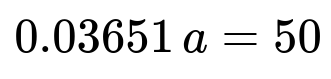
a × Φ(−2.5) + (1/2) a [Φ(−1.5) − Φ(−2.5)] = a × 0.03651.

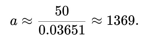
Setting this equal to 50 yields a = 50 / 0.03651 ≈ 1369.

Comprehensive Explanation

The goal is to find the value of a such that the insurance payout has an expected value of 50. We denote by X the random variable representing the item’s lifetime in years, with X ~ Normal(mean=7, std=2). The insurance pays a dollars if failure occurs in years 1 or 2, pays (1/2) a dollars if failure occurs in years 3 or 4, and pays 0 if failure occurs after year 4.

To compute the expectation, we note that:

E[Payment] = a times the probability that X ≤ 2 plus (1/2) a times the probability that 2 < X ≤ 4.

In more precise notation:

We must express these probabilities in terms of the cumulative distribution function (CDF) of the standard normal, which we denote by Φ. Since X is Normal(7,2), the probability that X ≤ x is Φ((x − 7)/2). Therefore,

• P(X ≤ 2) = Φ((2 − 7)/2) = Φ(−2.5).

• P(2 < X ≤ 4) = Φ((4 − 7)/2) − Φ((2 − 7)/2) = Φ(−1.5) − Φ(−2.5).

Substituting these into our expectation formula:

Numerically, one finds that

Φ(−2.5) ≈ 0.00621 Φ(−1.5) ≈ 0.06681 Φ(−1.5) − Φ(−2.5) ≈ 0.06060

Hence,

a × 0.00621 + (1/2) a × 0.06060 ≈ a × 0.03651.

We want E[Payment] = 50, so we solve for a in the equation:

which gives

Thus, setting a ≈ 1369 satisfies the requirement that the expected payout is 50.

Potential Follow-up Questions

How would the result change if the standard deviation were different?

One would re-compute the probabilities P(X ≤ 2) and P(2 < X ≤ 4) using the new standard deviation. The general formula for P(X ≤ x) with a Normal(mean=7, std=sigma) would be Φ((x − 7)/sigma). This changes the numeric values of Φ(...) in the expression for E[Payment], which would lead to a different multiplier on a, thus changing the final result for a when we set the expected payment to 50.

Why can we directly use the CDF of the standard normal distribution?

Whenever we have X ~ Normal(mean=μ, std=σ), any probability of the form P(X ≤ x) can be written as P((X−μ)/σ ≤ (x−μ)/σ). Since (X−μ)/σ follows the standard normal distribution, the probability P(X ≤ x) becomes Φ((x−μ)/σ). This is the standard technique for handling probabilities under any normal distribution and is a key reason for why tables or libraries for Φ are so widely used.

What if we wanted to adjust the payment structure to be continuous after the first two years rather than just up to four years?

We would define a piecewise payment function that depends on the specific year of failure, for instance a linearly decreasing function from full payment a up to zero by some cutoff time. Then, to find E[Payment], we would integrate over the probability density function of X multiplied by the corresponding payoff in each time interval. The core idea remains the same: the expected payout is always the integral of the payment function multiplied by the probability density function of X.

Could we have solved this using integration instead of the CDF?

Yes. You could explicitly write the expected payment as an integral of the form

integral over x of payout(x) f_X(x) dx,

where f_X is the normal probability density function. For instance, from x=0 to x=2, you pay a, from x=2 to x=4, you pay (1/2) a, and from x=4 to infinity, you pay 0. Splitting this integral or expressing it piecewise would lead to the same numeric result, but using the CDF Φ often simplifies the calculation for intervals of a normal distribution.

Below are additional follow-up questions

What if the insurance company wants to impose a maximum payout cap regardless of the value of a?

In some real-world scenarios, an insurance company might decide that no matter what, the maximum amount they pay for a single claim cannot exceed some fixed upper bound, say M. This scenario introduces an additional constraint:

• If a (the chosen payout for early failure) exceeds M, then effectively the insurance would pay only min(a, M).

• Similarly, for partial payments like (1/2) a, the cap would also imply a max payout of min((1/2) a, M).

Detailed Explanation

When a maximum cap M is imposed, you can no longer simply compute the expected payment as a × P(X ≤ 2) + (1/2) a × P(2 < X ≤ 4). Instead, you must consider the event that the required payout a (or (1/2) a) exceeds M. For instance:

• If a > M, the actual payment is M for the first two years, not a.

• If (1/2) a > M, the actual payment is M for the third and fourth years.

You would therefore break down the expected value of the payout into regions:

1. If a ≤ M and (1/2) a ≤ M, then no cap is actually triggered, so the formula remains the same.

2. If a > M but (1/2) a ≤ M, then for X ≤ 2, the payout is M, but for 2 < X ≤ 4, the payout is still (1/2) a.

3. If a > 2M, that implies (1/2) a > M as well, so both tiers would be capped at M.

In each situation, the expected payment formula changes accordingly, and you solve for a subject to whichever region you fall under. This leads to piecewise conditions for a. One subtle pitfall is that you might end up with no solution if the desired expected payout (for example, 50) is smaller or larger than what the cap structure can produce at feasible values of a.

How can we incorporate a deductible where the insurance pays only after a certain threshold time?

Insurance often has a deductible-like mechanism where small “failures” (e.g., failing in the first year) might not be fully covered unless it exceeds some threshold T. One might say: “The item must survive at least T years before coverage starts.” That is, if the item fails prior to T, there is zero payout, and coverage starts only after T.

Detailed Explanation

This scenario reverses the original structure. Instead of paying more for early failures, the insurance might pay more only if the item fails after T years. You would:

1. Define T as the threshold year beyond which payouts apply.

2. Decide on the new structure (e.g., from T to T+2 years, pay a, from T+2 to T+4 years, pay (1/2) a, etc.).

Mathematically, you would compute probabilities P(T < X ≤ T+2), P(T+2 < X ≤ T+4), and so forth, always using the normal distribution with mean 7, std 2. Then, the expected payment becomes the sum of those probabilities times their respective payouts. One subtlety is ensuring T is nonnegative (you can’t start coverage at negative time) and also verifying that T does not exceed the mean so much that the probability of paying becomes too small to be meaningful. In real life, the insurer carefully calibrates T to balance competitiveness and profitability.

Could partial failures or multiple partial payouts occur instead of a single payout?

Sometimes an insurance policy is structured so that each year (or each half-year) after an initial period might trigger partial payouts if certain “failure” conditions are met. For example, certain product warranties might pay a fraction of the replacement cost depending on how many months have elapsed.

Detailed Explanation

In such a case, we no longer have just two or three time windows. Instead, the payout function can become more granular, perhaps a continuous function of time:

• Payment(t) = a function that decreases with t, for instance linearly or stepwise over time.

To compute the expected payout, you would integrate Payment(t) multiplied by the probability density function of the normal distribution from t = 0 to infinity. Symbolically,

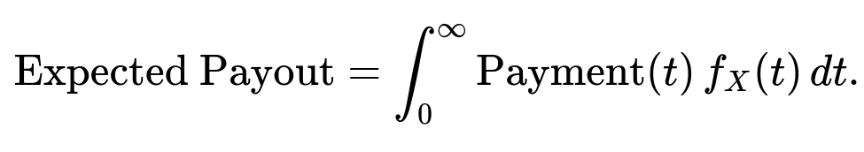
where f_X(t) is the normal density with mean 7 and std 2. You can approximate it numerically or sometimes find a closed form if Payment(t) is piecewise linear. A pitfall is to ensure the Payment(t) function is well-defined for all t≥0 and that it matches the intent of how partial payouts accumulate across time.

What if the lifetime distribution is not normal but log-normal or gamma distributed?

The normal assumption might be an oversimplification, especially for lifetimes, which are strictly nonnegative and can be skewed. Many engineering and biological processes are better modeled with a log-normal or gamma distribution.

Detailed Explanation

1. Changing Distribution If X follows a log-normal distribution with parameters (μ, σ), then ln(X) is normally distributed with mean μ and std σ. The probability P(X ≤ x) for x>0 becomes P(ln(X) ≤ ln(x)) = Φ((ln(x)−μ)/σ). In the gamma distribution, you have shape and rate (or scale) parameters, and you would compute probabilities from the gamma CDF.

2. Recomputing Payouts The same structure remains: pay a for X ≤ 2, pay (1/2) a for 2 < X ≤ 4, else 0. But now each probability is computed using the new distribution’s CDF. For instance, if X is log-normal, you evaluate log(2) in place of 2, and so on.

3. Edge Cases If the distribution is heavily skewed, the chance of failing before 2 years could be much smaller or larger than in the normal model. This drastically changes the value of a required to achieve an expected payout of 50. A potential pitfall is incorrectly applying normal-based tables or approximations to a nonnormal distribution, causing serious mispricing of the insurance product.

How would the solution differ if there is a minimum guaranteed payment?

Consider the scenario where the insurance contract promises a minimum payout of m dollars no matter when the item fails. That is, even if it fails after year 4, the insurer still pays m (though the rest of the structure might remain the same for earlier failures).

Detailed Explanation

1. Revised Payout

   • Fail by year 2: max(a, m)

   • Fail between year 2 and 4: max((1/2) a, m)

   • Fail after year 4: m

2. Expected Payment Formula Let p1 = P(X ≤ 2), p2 = P(2 < X ≤ 4), p3 = P(X > 4). Then

   E[Payment] = p1 × max(a, m) + p2 × max((1/2) a, m) + p3 × m.

   This can be broken into cases depending on whether a and (1/2) a exceed m. If a ≤ m, then effectively you are always paying m in the first two years. If (1/2) a ≤ m, then you also pay m for the 2–4 window, etc. You solve the resulting piecewise system for a so that E[Payment] = 50.

3. Pitfalls Similar to the maximum cap scenario, you can have piecewise conditions depending on whether a≥m or a<2m, etc. Each region might change your formula for the expected payout. You must handle these carefully or risk an incorrect a value.

How would we approach the problem if there is a waiting period before coverage starts?

An insurance policy might stipulate that coverage only begins after 1 year (waiting period). That means if the item fails within that waiting period, there is no payout, even if it is within the 1–2 year window.

Detailed Explanation

If the waiting period is 1 year, you effectively shift the coverage windows:

• For t ≤ 1, Payment = 0.

• For 1 < t ≤ 2, Payment = a.

• For 2 < t ≤ 4, Payment = (1/2) a.

• For t > 4, Payment = 0.

Now you compute:

1. P(1 < X ≤ 2) = Φ((2 − 7)/2) − Φ((1 − 7)/2).

2. P(2 < X ≤ 4) = Φ((4 − 7)/2) − Φ((2 − 7)/2).

3. P(X ≤ 1) and P(X > 4) lead to zero payout.

Then the expected payout formula modifies accordingly:

E[Payment] = a × P(1 < X ≤ 2) + (1/2) a × P(2 < X ≤ 4).

As before, set that equal to 50 and solve for a. However, you will get a different numeric solution because the coverage interval for the full payout a is now only from 1 to 2 years, which typically has a higher survival probability than from 0 to 2. A subtlety is that the definition of “year of failure” might not match cleanly with the waiting period in real contracts, so you must be precise in how these intervals overlap.

What if the insurance cost a must also include the expense ratio and profit margin of the insurer?

In practice, the premium the insurer charges for coverage is not exactly the expected payout; they add loadings for administrative expenses, risk margins, broker commissions, etc. Suppose the insurer wants the expected payout to be 50, but they must set a premium that is 50 / (1 − expense_ratio) to account for overhead.

Detailed Explanation

1. Expense Ratio If the expense ratio is r (e.g., 20%), that means for every 1 dollar of premium, 20% goes to expenses, so only 80% is left for claims.

2. Premium vs. a Let’s say the insurance company sets the premium P, and from that premium, they want to pay out an expected 50. Then P * (1 − r) must equal 50. So P = 50 / (1 − r).

3. Relation to a We found that 50 = 0.03651 × a in the normal scenario. So a = 50 / 0.03651. But in real life, the insurer must ensure the premium minus expenses is sufficient to cover that 50. So if the insurer sets a purely for the coverage, they might then realize the premium must be higher to cover overhead.

A pitfall is failing to realize that a is the coverage-level parameter, whereas the premium the policyholder actually pays might be a separate figure that includes overhead. In interviews, highlighting how the real-world premium is usually higher than just the “fair” expected payout underscores an understanding of practical insurance pricing.

What happens if we only have empirical data rather than a theoretically assumed normal distribution?

In many data-driven contexts, the distribution of X is inferred from sample data on past item lifetimes. We might not know that it’s exactly normal or log-normal. Instead, we have empirical data that we can use to estimate probabilities.

Detailed Explanation

1. Empirical Distribution Instead of P(X ≤ 2) = Φ((2−7)/2), you approximate P(X ≤ 2) by the proportion of historical items that failed by year 2. Similarly for P(2 < X ≤ 4).

2. Monte Carlo or Nonparametric Estimation

   • You could do a Monte Carlo simulation or a direct nonparametric estimate from the empirical cumulative distribution function (CDF).

   • Then compute E[Payment] = a × p1 + (1/2) a × p2, where p1 and p2 come from data.

3. Pitfalls

   • Sample size might be too small, leading to imprecise estimates.

   • Real distribution might change over time (non-stationarity) or vary with manufacturing improvements, so old data might not represent future lifetimes.

   • Outliers in lifetime data could skew the estimates of early or late failures.

A thorough approach might combine domain knowledge (e.g., typical mechanical wear-out distributions) with statistical analysis (e.g., robust estimation methods) to come up with the best possible model for X.