
ML Interview Q Series: Devil's Penny Problem: Maximizing Expected Winnings via an Optimal Stopping Threshold.

Browse all the Probability Interview Questions here.
You have eleven closed boxes in front of you, arranged in random order. One box contains a devil’s penny, and the other ten contain known dollar amounts a_1, …, a_10. You can open as many boxes as you like, one at a time. You get to keep the total money from all the boxes you have opened, provided that none of them contained the devil’s penny. The moment you open the box with the devil’s penny, the game ends and you lose all the money you have collected so far. What is a good stopping rule to maximize the expected value of your winnings?
Short Compact solution
A simple and optimal threshold strategy is to stop opening boxes as soon as the total amount you have collected reaches at least half of the sum A = a_1 + a_2 + ... + a_10. Formally, if a denotes the sum of the amounts you have already collected from opened boxes, you stop as soon as a ≥ (1/2)A. Otherwise, if a < (1/2)A, you continue opening more boxes.
Comprehensive Explanation
One-stage look-ahead argument
This problem can be analyzed using a one-stage look-ahead principle. At any point in time, let:
k+1 be the number of remaining unopened boxes (including the one possibly containing the devil’s penny).
a be the total amount you have collected so far (from the boxes that did not contain the devil’s penny).
A = a_1 + a_2 + ... + a_10 be the total sum of the ten dollar amounts across all safe boxes.
We define X_k(a) as the random variable describing the net gain (change in total capital) if you decide to open one more box given that you currently have a dollars. In other words, X_k(a) captures how your total collected amount changes after deciding to open the next box.
A key insight is that if the expected value of X_k(a) is positive, then it is beneficial to open another box. If the expected value of X_k(a) is non-positive (i.e., ≤ 0), then opening another box no longer increases your expected gain, so you should stop.
Expected value of opening one more box
We want to compute the expected change in your total amount if you choose to open an additional box when you already have a dollars. Among the k+1 unopened boxes, one has the devil’s penny, and the other k contain the amounts from the set {a_i1, ..., a_ik}, which are some subset of the original a_1, ..., a_10.
The probability of hitting the devil’s penny in the next draw is 1/(k+1), in which case you lose the entire collected sum a. The probability of hitting one of the safe boxes is k/(k+1), in which case you gain the average of the amounts in those k safe boxes. Because the total remaining dollars in the safe boxes is (A - a), and they are uniformly likely among the k boxes, the average amount you might gain if you pick a safe box is (A - a)/k.
Putting it together, a well-known derivation (and also a more formal approach using the conditional expectation) shows that:
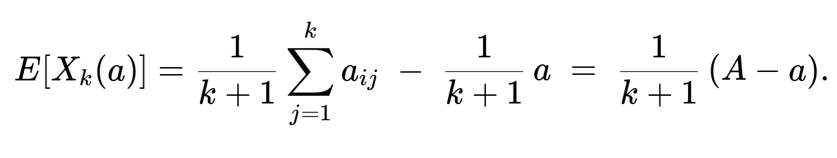
Here:
(1/(k+1)) * sum_{j=1..k}(a_{ij}) = average gain if you pick one of the k safe boxes.
(1/(k+1)) * a = the expected loss from the risk of drawing the devil’s penny (which costs you your entire current sum a).
Hence the net effect is (1/(k+1)) (A - a).
Stopping criterion
We compare E[X_k(a)] to zero:
So once the amount a you have collected so far exceeds or equals (1/2)A, the expected change from continuing is no longer positive. Therefore, the one-stage look-ahead rule says you should stop as soon as a ≥ (1/2)A. If a is less than (1/2)A, the expected value of opening another box is still positive, and you continue.
Intuition behind the threshold at A/2
The threshold emerges from balancing the risk of losing everything against the chance of boosting your total winnings with the remaining safe boxes. If you already have half of the sum of all dollar amounts, the “upside” from picking more boxes (given that one box is the devil’s penny) no longer justifies the downside of possibly losing all a dollars. This threshold is entirely distribution-agnostic (it does not matter which boxes contain large or small amounts) as long as you only know the sum A and your current total a.
Follow-Up Question 1
Why doesn’t the exact distribution of the amounts in the unopened boxes matter, beyond knowing their sum?
The reasoning hinges on the linearity of expectation and the fact that once you have the partial sum a, the “missing” amounts (A - a) must be spread across the unopened safe boxes. Since only one unopened box is “bad” (the devil’s penny), the remaining expected payoff from those safe boxes primarily depends on (A - a), not on how (A - a) is distributed. The one-stage look-ahead calculation averages out any differences in individual box contents.
Follow-Up Question 2
Could there be a scenario where a more intricate strategy (e.g., picking certain boxes based on prior knowledge) improves on the A/2 rule?
If the placements of amounts were known or you had some partial knowledge (say, you know some boxes are likely to have bigger amounts), you might attempt a more sophisticated approach. However, in the problem’s standard formulation, the boxes are in a random order with no a priori correlation between their positions and the amounts they hold. You only track your current total a. As a result, the threshold rule at (1/2)A remains optimal under the stated assumptions. If more information were available (for instance, if you had partial knowledge of which boxes contain certain sums), the strategy might change.
Follow-Up Question 3
Is there a simple way to simulate and verify this stopping rule in a programming language?
Yes, you can use a Monte Carlo simulation to empirically compare different stopping rules. For instance, you can implement the game with random permutations of the boxes (one containing the devil’s penny, the others containing the a_i amounts) and then simulate multiple runs with different strategies.
Here is a simple Python example:
import random
import statistics

def simulate_game(a_amounts, n_sim=10_000):
    A = sum(a_amounts)
    half_threshold = 0.5 * A
    gains = []
    for _ in range(n_sim):
        # Randomly place one devil's penny among the amounts
        boxes = a_amounts + [None]  # None signifies devil's penny
        random.shuffle(boxes)

        current_sum = 0
        for box in boxes:
            # Check if we should stop
            if current_sum >= half_threshold:
                break
            # Open next box
            if box is None:
                current_sum = 0  # Lost everything
                break
            else:
                current_sum += box

        gains.append(current_sum)

    return statistics.mean(gains)

a_amounts_example = [10, 30, 5, 40, 15, 25, 10, 10, 20, 35]
expected_gain = simulate_game(a_amounts_example, n_sim=100000)
print("Estimated expected gain:", expected_gain)
In this simple code:
a_amountsis the list of the 10 positive amounts.We add one
Noneto represent the devil’s penny.We shuffle the list (randomly permuting it).
We keep opening boxes until we either hit the penny (None) or our sum ≥ (1/2)A.
We collect results and compute the mean.
You can experiment with different rules—for example, always open all boxes, or open only two boxes, etc.—and compare their empirical expected values. You will typically find that the half-of-total-sum strategy holds up very well (and matches the theoretical analysis).
Below are additional follow-up questions
Follow-up Question 1
What if the total sum A is not precisely known, but we only have an estimate or a distribution for it?
When A is uncertain, the threshold strategy “stop when a >= 0.5 A” must be adapted because we do not know the exact half point. One potential approach is to replace the unknown A with its expected value E(A). Then, the stopping rule becomes “stop when a >= 0.5 E(A).” However, this can be suboptimal if the variance in A is large. A more nuanced strategy might incorporate Bayesian updating of our belief about A as we open boxes. For instance, each newly opened safe box reveals partial information about how large the remaining sum could be. In real-world scenarios, ignoring that uncertainty can lead to either stopping too soon (if A turns out to be bigger than expected) or pushing your luck too far (if A is overestimated). A thorough solution might require formulating a Bayesian prior on the amounts a_1, ..., a_10, updating that prior with each revealed box, and computing the expected net gain from opening the next box under the updated distribution.
Pitfalls / Edge Cases:
If our initial estimate of A is heavily biased, we may repeatedly make a suboptimal decision to continue or stop.
If the actual distribution of the amounts is heavier-tailed (higher chance of large sums) than our assumption, we might forgo large gains by quitting too early.
If some domain knowledge strongly suggests an upper or lower bound on A, we should incorporate that knowledge rather than assume it is unbounded.
Follow-up Question 2
How does risk aversion or a utility function different from pure expected value impact the stopping rule?
In many real-world settings, maximizing the raw expected value is not the sole objective; risk-averse players may prefer a strategy that lowers variance or avoids catastrophic loss. If your utility is non-linear—say, U(x) = log(x)—the threshold strategy changes because losing the entire current sum is much more damaging in terms of utility than it is in a purely linear expectation sense. Typically, a risk-averse utility function encourages earlier stopping to avoid a sharp drop in utility if the devil’s penny is revealed.
Pitfalls / Edge Cases:
Different utility functions can produce dramatically different decisions. For example, with a strongly concave utility function, you might stop opening boxes as soon as you gain even a small fraction of A.
In practice, defining the “true” utility function might be difficult; if you approximate or guess it incorrectly, your stopping rule might fail to meet your real objectives.
Follow-up Question 3
What if each safe box can contain a potentially negative value, representing a net cost rather than a gain?
In some variants of this problem, the “box amounts” might include debts or negative payouts. If negative values are allowed, then A = a_1 + ... + a_10 might be less than zero, or some partial sums a might decline upon opening a certain box. The one-stage look-ahead argument still applies: you compare the expected increase from opening another box against the risk of losing what you have. However, the threshold that emerges from E(X_k(a)) ≥ 0 would differ if A < 0 or if the distribution of box values is mixed between positive and negative. You might even be willing to open more boxes if your current sum is negative (since losing a negative amount is actually beneficial in some interpretations—though that depends on the exact game setup rules).
Pitfalls / Edge Cases:
If A < 0, the sign of the expected incremental gain from opening boxes can flip more easily, possibly prompting the player to open boxes indefinitely.
The notion of “losing all the money you have so far” might need reinterpretation if your total is already negative. Some game designs might treat negative amounts differently, so clarifying the payoff structure is essential.
The formula for E(X_k(a)) continues to hold, but the threshold at which it is zero might become a negative fraction of A, or might not be a meaningful stopping point in practical terms.
Follow-up Question 4
In an extended version, suppose you are given a limited option to skip opening a certain number of boxes without revealing them. How might this affect the threshold strategy?
If the game allows skipping boxes without penalty but you still have to open them in a specific sequence, your strategy might shift. For instance, you could choose to skip boxes that you suspect might have small amounts (if you have any such heuristic) or skip randomly to reduce the risk of encountering the devil’s penny until you have a more favorable state. However, if the location of the devil’s penny is equally likely in all unopened boxes, skipping does not directly reduce the probability of hitting the devil’s penny in the next actual opening—it merely delays it.
A rational approach would evaluate the expected value of skipping a box: does it improve the conditional chance that the next box you open has a sufficiently large amount relative to the risk? Under purely random distribution with no additional information, skipping typically does not yield any strategic advantage over deciding whether or not to open the next box. You would still fall back on a threshold rule for how much you have gained so far.
Pitfalls / Edge Cases:
If skipping changes probabilities in a subtle way (e.g., if there is partial information about which box might contain the devil’s penny), then skipping could become valuable.
Complexity grows if you also have partial knowledge or can choose the order in which boxes appear after skipping some. In that case, the problem might require dynamic programming or more advanced Bayesian approaches to find the optimal strategy.
Follow-up Question 5
What if the player can purchase “insurance” to protect a portion of their current sum if they open the devil’s penny?
An interesting twist is allowing the player to pay a fee at certain stages to protect or lock in some of their gained amount. In effect, if they open the devil’s penny after buying insurance, they keep a guaranteed portion of their sum. This scenario introduces a decision layer where you weigh the insurance cost against the potential gain from continuing.
Analyzing this scenario involves comparing:
The updated expected gain if you pay for insurance and continue opening boxes.
The expected loss you might incur without insurance.
The fraction of your sum that remains protected after you hit the devil’s penny.
The stopping rule might then become “stop once the expected additional gain minus the cost of insurance is no longer positive,” which is reminiscent of the original threshold logic but factoring in an extra cost (the insurance premium).
Pitfalls / Edge Cases:
If insurance is overpriced relative to the expected incremental gain, buying it is detrimental.
If the cost is small but covers a large fraction of your sum, it might be always beneficial to purchase it and continue opening boxes until you reach a higher threshold.
Calculating the “fair value” of insurance can be tricky, especially if the game includes partial knowledge or complicated distributions of box amounts.
Follow-up Question 6
Could the order in which boxes are opened matter if the devil’s penny is not uniformly distributed but correlated in some way with the amounts?
In the standard problem, the devil’s penny is assumed to be equally likely in any of the eleven boxes, independent of the dollar amounts in each. If there is any correlation—say, the devil’s penny is more likely to be in boxes with higher amounts or is in a box that is physically heavier—then the assumption of uniform randomness fails. You might glean information from partial observations about which boxes are more or less likely to contain the penny, altering your expected payoff calculation. This would demand a more complex strategy that updates beliefs after each opened box (e.g., a Bayesian approach if certain distributions and correlations are known).
Pitfalls / Edge Cases:
Even a slight correlation can drastically change the risk profile. For instance, if high-value boxes are more likely to contain the devil’s penny, you might want to open boxes that seem smaller first, hoping to accumulate a risk-free sum.
Without precise knowledge of the correlation, you could make incorrect assumptions that diminish expected gains.
If the correlation is in your favor (e.g., the devil’s penny is more likely in a low-value box), a naive approach might open the high-value boxes first, ironically maximizing risk unless you quantify that correlation carefully.
Follow-up Question 7
How would the strategy change if you knew in advance that you must open a certain minimum number of boxes regardless of your total so far?
If the rules say you are obligated to open, say, at least 3 boxes, you cannot stop before you have opened 3. In that case, the threshold rule starts to apply only after you fulfill the mandatory opening requirement. Up to that point, you have no choice but to open boxes. Once you have opened the required minimum, you can evaluate how much you have collected so far and compare it to the threshold. If you have met or exceeded the threshold by then, you stop immediately. Otherwise, you keep going if the expected value from continuing is positive.
Pitfalls / Edge Cases:
If you are forced to open a certain number of boxes, you risk immediately hitting the penny and ending up with zero. This might reduce the overall expected gain compared to the unconstrained scenario.
If the forced openings are fewer than the expected number of boxes you would normally open in the threshold strategy, it may not hurt you too much. But if it is a larger number, you might be forced to continue well beyond your original threshold, raising your chance of losing everything.
You must decide how to choose which boxes to open during the forced stage—though in the standard random arrangement model, you typically have no knowledge that would give one box a higher or lower devil’s penny probability than another.
Follow-up Question 8
What if partial winnings are locked in periodically, rather than lost entirely upon finding the devil’s penny?
In some game variants, you might forfeit only a fraction of your current sum if the devil’s penny is drawn. For example, you lose half of what you have instead of everything. This changes the expected cost of continuing. The one-stage look-ahead formula modifies to reflect the partial forfeit rather than total loss. Specifically, if your new capital after hitting the penny is not zero but some fraction of a, the risk is less severe. You might open more boxes on average because the downside is not as catastrophic.
Pitfalls / Edge Cases:
The exact fraction lost upon hitting the penny drastically alters the threshold for continuing. If the loss is small, you might continue until a is close to A.
If the fraction changes dynamically (e.g., you lose 90% of your current sum if you open the penny after the 5th box, but 50% if it happens later), the stopping rule can become quite complicated. You would need to do a more advanced expected value analysis that accounts for variable loss rates.
In real implementations, ensuring the correct formula for partial forfeiture is used is crucial. A mistake here leads to an incorrect threshold.
Follow-up Question 9
Does the presence of very large outlier amounts among the a_i significantly affect the threshold approach?
If one or two of the a_i are extremely large compared to the others, one might wonder if you should keep opening boxes until you hit one of these big amounts, even if you have already reached half of A. However, the half-of-A threshold is based on the expectation of what you gain vs. the risk of losing what you have. Even if one box is huge, the probability of hitting the devil’s penny might offset the potential benefit of chasing that large prize. Mathematically, the one-stage look-ahead approach still incorporates the entire sum A, so the threshold of 0.5 A remains valid for a uniform risk.
Pitfalls / Edge Cases:
If the distribution of a_1, ..., a_10 is extremely skewed, the incremental expected gain from opening another box might feel compelling, but the risk of losing a significant current sum might still outweigh this unless you have further details (e.g., knowledge that the largest box remains unopened).
Real-life decision-makers may be tempted to “gambler’s fallacy” if they see many small boxes opened already, believing the large one is more likely to appear. But in truly random scenarios, each remaining unopened box is still equally likely to be the devil’s penny.
Follow-up Question 10
How important is computational efficiency if we were to solve a more complex or generalized version of this problem with many more boxes?
In practice, one might generalize this game to far more than ten safe boxes plus one devil’s penny. For large numbers of boxes (like 100, 1000, or more), an exact dynamic programming approach could become computationally expensive. However, the simple threshold rule that emerges from the one-stage look-ahead principle scales very naturally. You merely keep track of how much you have accumulated so far vs. the total sum A. This avoids the combinatorial explosion that might occur if you tried to calculate all possible sequences of box openings.
Pitfalls / Edge Cases:
If the problem is extended to large-scale variants with partial information or correlated distributions, you might need approximate methods (e.g., Monte Carlo simulations, approximate Bayesian updates, or heuristics) to guide the stopping rule.
A naive dynamic programming approach for many boxes might be infeasible due to exponential state space, reinforcing the appeal of threshold-based methods that are computationally simple and yet near-optimal (or exactly optimal under uniform assumptions).
Implementation details (like tracking which boxes remain, updating partial sums, etc.) might introduce complexity, but the basic threshold logic still helps you determine “open vs. stop” in a straightforward manner.