
ML Interview Q Series: Dice Game Payouts: Analyzing Product vs. Square with Expected Value and Variance.

Browse all the Probability Interview Questions here.
You have two different dice games to choose from. In the first, you roll two dice together and earn a payout equal to the product of their faces. In the second, you roll a single die and receive the square of that face as your payout. Which of these two games has the higher expected payoff, and what is the reason behind it?


Illustrative Python Code
Below is a short Python snippet that estimates these values through simulation:
import random
import statistics

def simulate(num_simulations=10_000_000):
    product_payouts = []
    square_payouts = []

    for _ in range(num_simulations):
        # Game 1: Roll two dice
        d1 = random.randint(1, 6)
        d2 = random.randint(1, 6)
        product_payouts.append(d1 * d2)

        # Game 2: Roll one die
        d_single = random.randint(1, 6)
        square_payouts.append(d_single ** 2)

    return statistics.mean(product_payouts), statistics.mean(square_payouts)

avg_product, avg_square = simulate()
print("Estimated E[product of two dice]:", avg_product)
print("Estimated E[square of one die]:", avg_square)
If you run enough simulations, you should see that the average product hovers near 12.25, while the average square is near 15.17, which matches the theoretical results.


Could machine learning or deep learning approaches help in analyzing dice games?
Machine learning typically comes into play when dealing with complex, high-dimensional data or when the underlying distribution is unknown or unwieldy to compute analytically. For a simple dice game with known distributions, direct probability and mathematical reasoning is more efficient. However, if you had a complicated board game with many possible moves and dice rolls, you could use simulation-based approaches or reinforcement learning techniques to estimate long-term expected rewards under different strategies. But for these straightforward dice rolls, pure math is best.
If we changed the second game to rolling two dice and squaring their sum, would it still surpass the product?

Below are additional follow-up questions
How would the analysis change if each game came with an entrance fee or different costs to play?


Does risk tolerance or utility theory ever make you pick the game with the lower expected value?
In many real-life settings, a player’s risk appetite (or risk aversion) can influence which game they prefer. Classical expected-value comparisons assume that a gambler values a dollar of gain equally whether they already have a large or small sum. However, many people experience diminishing returns (for instance, a utility function that grows sub-linearly with money).
If someone is risk-averse, they might prefer a game whose payout distribution is more predictable, even if it has a slightly lower expected value.
Conversely, a risk-seeking individual might prefer games with higher volatility, especially if there is a chance for very large winnings.
Pitfalls and Edge Cases:

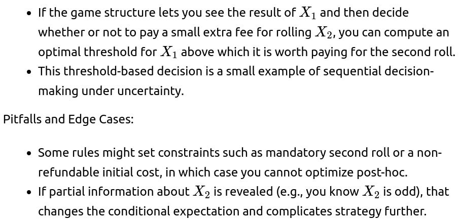
What if the dice in the first game are not rolled simultaneously, and you can decide whether or not to roll the second die?
If the game rules allow you to see the first die roll before committing to the second roll, you might adopt a strategy: if the first roll is too small, maybe you forfeit or choose not to roll the second die. However, typically in standard games, forfeiting means earning zero or some other minimal payoff.
How does the analysis change if you can roll the single die repeatedly and pick the highest square outcome?
In some variants of the second game, you might be allowed multiple attempts and take the best of those attempts. This changes the distribution significantly because the expected maximum of multiple die rolls is higher than the mean of a single roll.
Pitfalls and Edge Cases:
Each roll might come with an additional cost or constraint, so it may not be purely beneficial to keep rolling without limit.
In certain practical games, there might be a cap on how many re-rolls you get, or the best outcome might be forced after too many attempts.
If the dice in Game 1 are correlated instead of independent, how does that affect the expected product?
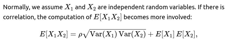
where ρ is the correlation coefficient. A positive correlation means we are more likely to see both dice show high numbers simultaneously (which might inflate the product). A negative correlation means large outcomes on one die are more likely to pair with small outcomes on the other (which typically reduces the product).
Pitfalls and Edge Cases:
Real dice used physically are generally close to independent, but mechanical irregularities or special manufacturing flaws could induce correlation.
In a contrived digital game, the developer might rig the outcomes to be correlated (positively or negatively) to create a certain distribution of products.
Are there practical scenarios where the maximum payout is capped, and how does that affect the comparison?
In many real-world gambling or board-game scenarios, there might be a maximum payout limit. For instance, you cannot win more than $20 in any roll or any single bet.
If Game 2 has a natural maximum payoff of 36 (rolling a 6), imposing a $20 cap might reduce its advantage because all outcomes that are 25 (square of 5) or 36 (square of 6) would just yield 20.
Meanwhile, Game 1’s product game also has a maximum theoretical payout of 36, but the distribution of high outcomes is different. So capping might reduce the difference between the two games.
Pitfalls and Edge Cases:
Once a payout ceiling is introduced, straightforward expectation calculations must adjust for truncated distributions. You would recalculate expected values under the cap:

What happens if we consider the median outcome or other statistics instead of the mean?
Sometimes, decision-makers care more about median or quantiles than average outcomes. This can be especially relevant in risk management contexts or certain game design scenarios.

Different percentile measures (like the 75th percentile) might yield alternative perspectives on which game has “better” typical payouts.
Pitfalls and Edge Cases:
Median-based decisions can lead to suboptimal expected gains if a player’s utility is purely linear. However, in real-world scenarios, guaranteed or “likely” outcomes might matter more than long-shot large payoffs.
If the distribution is heavily skewed, focusing on quantiles might tell a very different story than the mean.
Is there a scenario in which game designers might prefer the lower expected value game?
From the perspective of a casino or game designer, offering a game with a higher expected payout typically means they lose money in the long run. A casino might prefer to implement a game with a lower or break-even expected value from the house’s viewpoint.
In some cases, the second game might be more alluring to players because it offers a chance at bigger single-roll payoffs (like rolling a 6 to get 36). But if the average cost to the house is too high, they could tweak the rules—perhaps by changing payouts for certain rolls—to ensure profitability.
Alternatively, they might prefer the first game (product of two dice) as it naturally has a slightly lower theoretical average payout, meaning the house edge is more favorable if players pay a fixed cost to play.
Pitfalls and Edge Cases:
Player behavior often depends on how “exciting” the game feels, not just raw math. If a game with a higher expected return for the player also yields bigger short-term swings, it could attract more engagement.
Some regulatory environments require that the house maintain a certain minimum RTP (return to player), so the game’s parameters must be carefully balanced to comply with local gambling laws.
If the dice faces could include zero or negative numbers, how does that complicate the analysis?

If there is a bonus multiplier or penalty for rolling certain values, does that shift which game is better?
Some specialized dice games apply extra rules, such as “If you roll a 6, you get a 2x multiplier,” or “If you roll a 1, your payout is halved.” These rules systematically shift the distribution of outcomes.
For the product-based game, a bonus multiplier for rolling a 6 on either die can significantly raise the expected value because 6 influences the entire product.
For the square-based game, the effect of a multiplier on certain faces might be even more dramatic when squared (for example, rolling a 6 with a 2x multiplier yields 36×2=72).
Pitfalls and Edge Cases:
Overly generous multipliers might make the game unsustainable if it is meant to be profitable for an operator.
Penalties could reduce the variance if they apply only to extreme outcomes, or they could cut down the expected value drastically if they are frequent.
How important is simulation verification for more complex rule sets?
While mathematical derivations are typically clean and exact for simple dice scenarios, real-world games can pile on many special rules, side bets, bonus triggers, or correlated events. When an analytic solution becomes cumbersome, simulation can be crucial.
By simulating many rounds, you empirically approximate the expected payoff, distribution, and potential extremes (like maximum observed payout).
You can also perform sensitivity analysis by adjusting certain rule parameters (like multipliers or penalties) to see how the expected value, variance, and distribution shape respond.
Pitfalls and Edge Cases:
Simulations must be correctly implemented. Coding errors or insufficient sample sizes can produce misleading results.
Rare events (like rolling multiple 6s in a row if there is a large multiplier) may be underestimated if the simulation doesn't run enough iterations or doesn't adopt a variance-reduction strategy.


